When Is A Complex System Stable?
In biology, there are systems where small perturbations lead to the same broad result.
Imagine a garden of many plant species, each with multiple numbers of them. If I plucked just one plant from one species, would this cause a ripple effect that suddenly causes another plant to become dominant and takeover the garden? It’s unlikely.
This is a property of complex systems called stability. Stability is when you change something about a system slightly, and the system tends back to the same result. It doesn’t explode or runaway.
What conditions do we need for a complex system to be stable? Suppose we knew. If we found a stable system through experiment, we could then make deductions about other properties of it that must hold true. For example, if we found that a soil microbiome was stable, then might be able to put bounds about how strongly the microbes interact with each other.
Knowing the conditions would also be useful in practical cases like policy or pandemic prevention. If we knew that a model of pandemic infection in a classroom was stable, we could say things about how robust interventions might be to implementation error.
In this post I’ll describe what stability is and visualise an insanely cool result by Robert May in 1972 on random matrix theory applied to ecology.
Eigenvalues and Stability
How can we quantify what stability actually is?
Complex systems are described by a big system of differential equations.
$$ \frac { d \mathbf x } { d t} = F ( \mathbf x ) $$
One necessary condition for a stable system is that without any perturbing, it should say the same. So, we require at some point that the derivative is zero.
$$ 0 = F ( \mathbf x ^ * ) $$
But this isn’t sufficient for a system to be stable We want to know what happens when we change x* slightly. Does the system end up going back to x*, or is there a runaway scenario, like when you put a ball balancing on an upside down bowl?
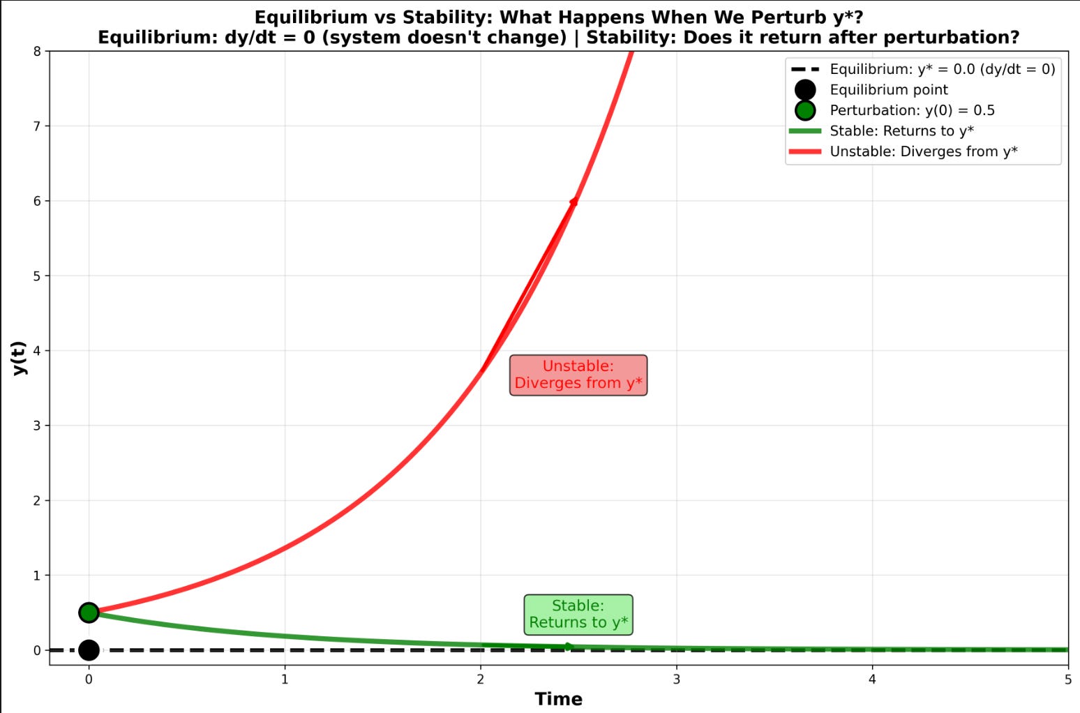
To figure out of the system comes back, we use a mathematical tricked called linearisation around the equilibrium point x*. To do this, we expand the F around the point in terms of it’s derivatives, and keep only the first order linear terms. This is a bit technical, and you don’t really need to know exactly how this works, but I’ve put the details below.
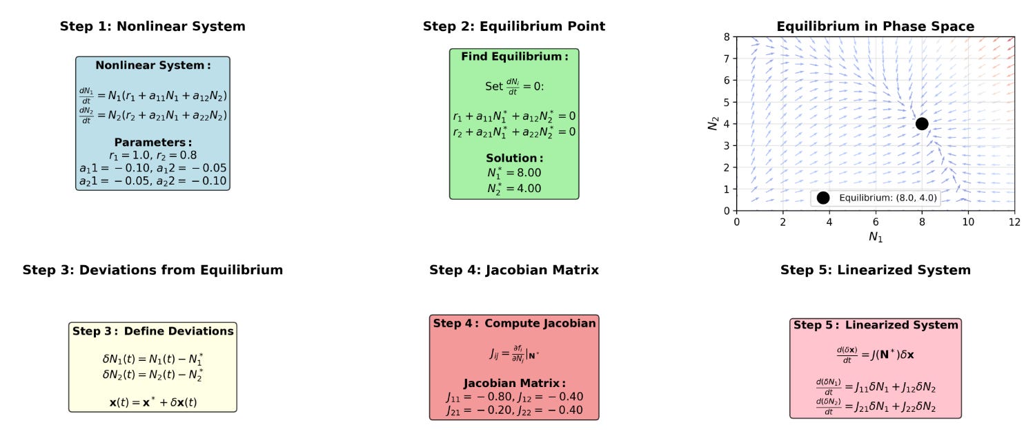
This procedure spits out is a matrix called the Jacobian. This matrix describes the dynamics of the system near x*, and allows us to rewrite the system as a linear one!
$$ \frac { d \delta \mathbf x } { dt } = J ( \mathbf x ^ * ) \delta \mathbf x $$
We know a lot about linear systems and their properties.
The most interesting thing about this linear matrix is its eigenvalues. Matrices transform vectors, but there are some vectors who remain invariant in their direction, but scale. Eigenvalues are how much these vectors scale by.
The eigenvalues of any matrix are complex, which means they are the sum of a real part and an imaginary part.
And most importantly, the eigenvalues determine the stability of a system.
Where these eigenvalues are on the real line determine whether a system is stable. If an eigenvalue has a positive real part, then that part of the system explodes. If it has a negative real part, then its stable! If it’s on the boundary, it’s called marginally stable, which we won’t cover for now.
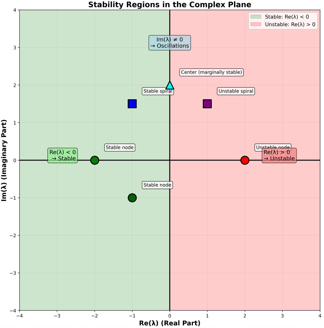
Different eigenvalues map to different trajectories. When the real part is negative, decay happens in the trajectory to a fixed value fairly quickly. If it’s’ positive, then a small perturbation causes the system to blow up exponentially. If there’s a non-zero imaginary component, then there will be some oscillation. I’ve plotted what the trajectories look like a 2 by 2 system here.
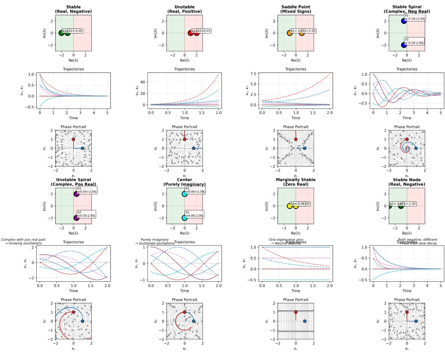
And so, a system is stable if all of its eigenvalues have a negative real part.
What About Real World Systems?
In most biological and chemical contexts, we have a lot of randomness and unknowns in our complex system. What happens when we have more than two species, and the elements of the matrix are random? Can we make any meaningful statements about its stability?
Lets look at the eigenvalues of a simple random system constructed by (May, 1972). May tried to find what the eigenvalues looked like for the random matrix A, where
$$ A = B - I $$
where I is the identity matrix and B is a random matrix. The elements of B are random variables with zero mean but a standard deviation alpha
$$ \begin{align} \langle B_{ij} \rangle &= 0 \\ \langle B_{ij}^2 \rangle &= \alpha^2 \end{align} $$
The animation below visualises what the matrix looks like as we increase alpha.
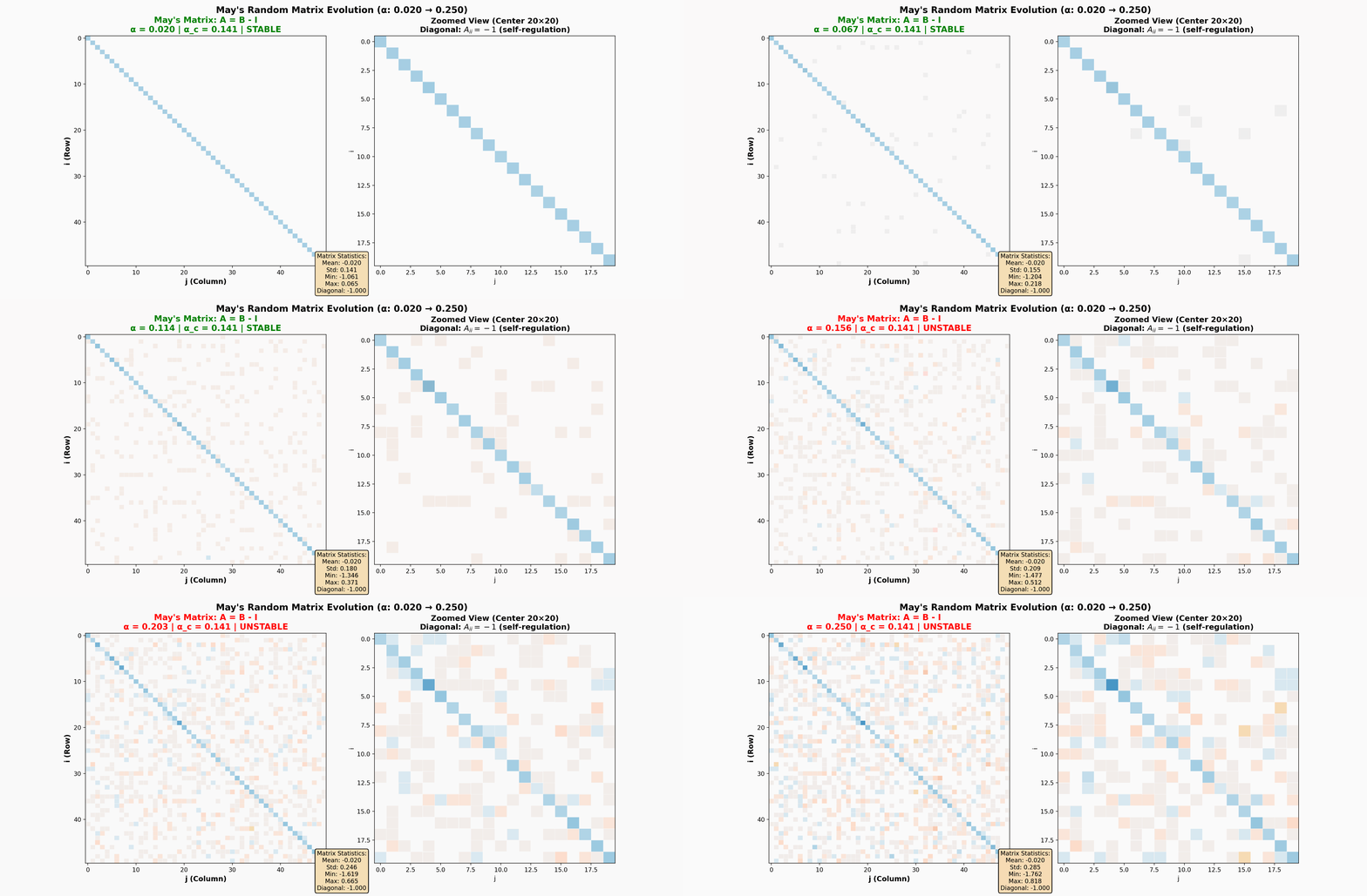
For a 50 by 50 matrix, let’s build this random matrix, plot the eigenvalues, and see what happens when alpha increases.
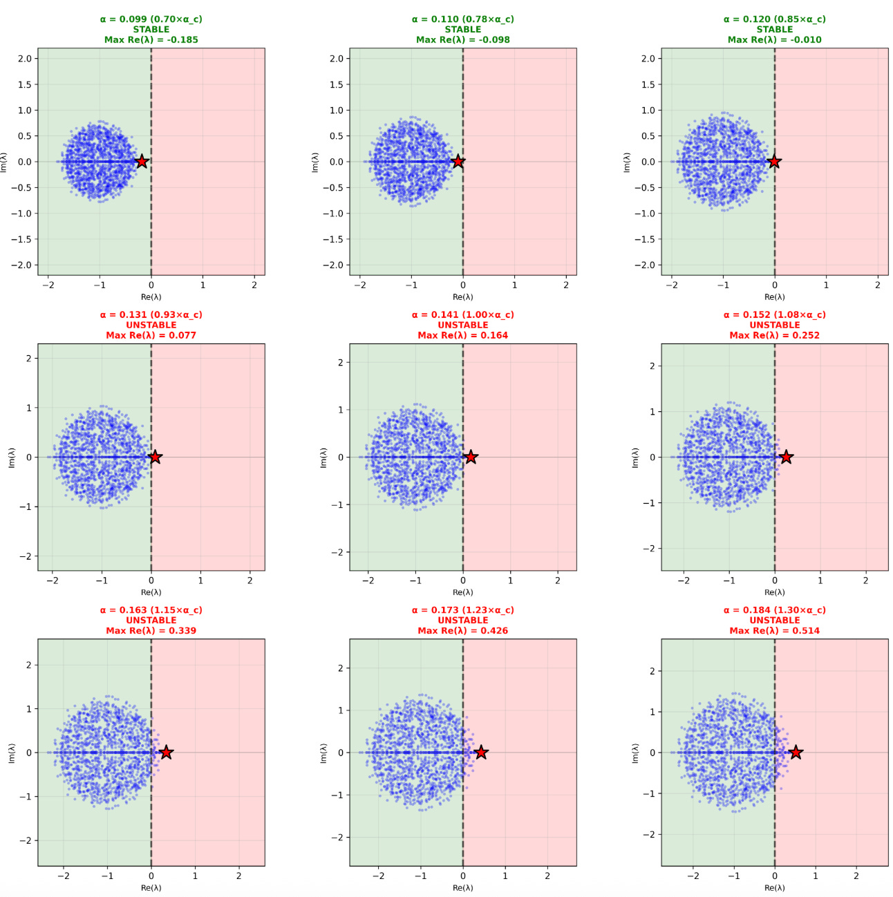
In the plots below, starting from the top left, I start with a small value of alpha, then plot its eigenvalues. At this level, all of the eigenvalues had a negative real part, and the largest real part of the eigenvalues was -0.185, which I’ve given a star. In this case, the system is stable, because all of the eigenvalues have a negative real part.
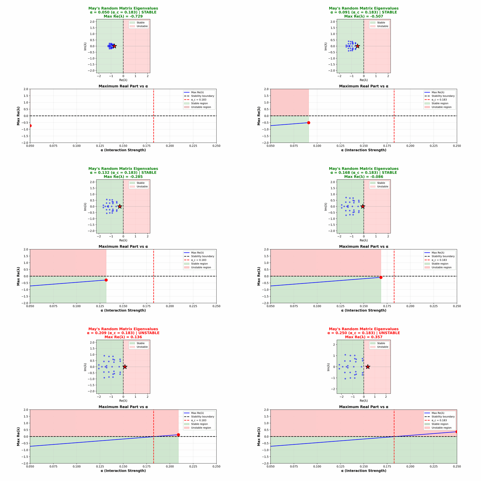
But when you increase alpha, the eigenvalues slowly disperse, until some cross into the positive real section. This is when the system ceases to be stable, because some of the eigenvalues have a positive real part.
I’ve visualised what happens as we increase alpha in this animation.
What value for alpha are we certain that a system described by a random matrix will be unstable?
I simulated this. For a given variance, I generated 200 random matrices. Then counted the number of matrices where all the eigenvalues have a negative real part as a fraction of the 200 matrices. On the left hand, I’ve plotted the probability that a matrix is going to be stable as a function of how high the variance is. I then did this for several different values of n, which is the size of the system.
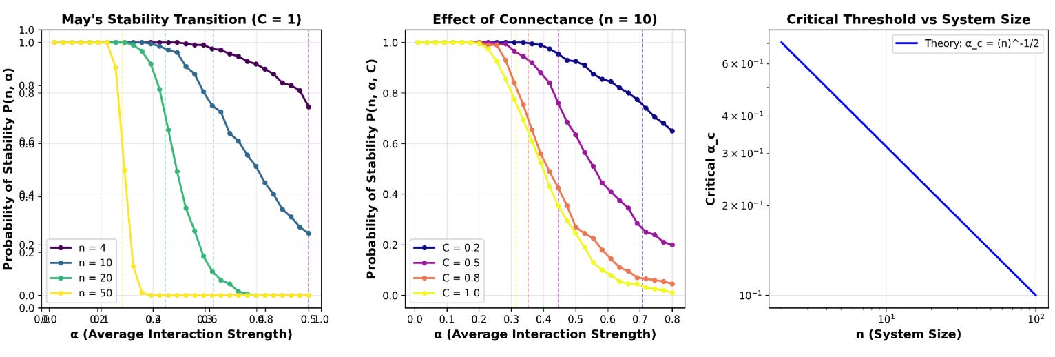
As alpha increases there is a sudden phase transition into a regime where the matrix is no longer likely to be stable. This happens at a critical value of alpha, which seems to depend on the size of the system n. You can see this transition behaviour in the yellow lines on the plot on the left, which sharply comes down when it passes the critical point.
As the size of the matrix increases, there is a smaller value of critical alpha at which the system is stable.
May worked out what the critical value is in May, R. M. (1972)! A system is almost certainly unstable when alpha is larger than inverse square root of n - the size of the matrix!
$$ \alpha_{c} = \frac { 1 } { \sqrt n } $$
I think this is an amazing result, and gives us an indication of what we can learn about variation in biology based on whether a system is stable. It also is a surprising link to concepts in statistical mechanics, like phase transitions.
Moving forward, I want to modify these types of systems and see if I can conjecture any other stability relationships that are interesting. There are also experiments that I want to test My first idea for testing this is getting multiple strains of bacteria from soil and then seeing how the competition between them evolves, and then checking to see if any biological parameters are consistent with the values in the stable regime.
References
May, R. M. (1972). Will a large complex system be stable? *Nature*, *238*(5364), 413-414.