Casual Physics Enjoyer

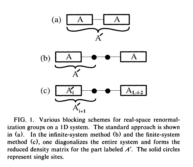
In the previous post, I outlined the shape of the Hamiltonian which governs this system. To find this ground state, we use the DMRG, and only restrict interactions to atoms which are sufficiently close. DMRG works by considering the ground state of only a small block of atoms and them iterating to mucn larger sizes. It’s the most precise algorithm to compute ground states in business right now.

To play with a simple toy example, let’s consider a chain of atoms which can either be in a spin-up, or spin-down state. The Hamiltonian in this spin chain contains a term which governs an interaction between two neighbouring atoms. The S is the spin operator, and it has three components since its a vector.

For large systems, diagonalising this Hamiltonian is near impossible. So, we need to find a numerical method to get just the low energy physics that we’re interested in.

What would be an initial approach to finding out this system?

Consider a system of length l, where l is very big. The Hilbert space consists of up or down states that could be in each one of these sites, and the energy is described by a Hamiltonian that is an operator on this Hilbert space. The energy eigenvalues of the Hamiltonian can be found by diagonalising this Hamiltonian, but this is an especially hard thing to do if the Hilbert space is very big. In this post, I'll outline a way to do this by diagonalising smaller blocks.

To remedy this issue, we divide up the problem into blocks. A block has a reduced Hilbert space, so it'll be easier to diagonalise and find energy eigenvalues. In the simplest case, we can combine the two Hamiltonians that we know, and then diagoanlise it. Then, with this large Hamiltoanian, we can truncate it into a reduced basis, to get a Hamiltonian that spans a bigger area but is the same size as the original block.

One of the systems in which the first method might work is a particle hopping between different sites. In this example, if we have L sites that a particle can occupy, then our Hilbert space has dimension L. In this Hilbert space, each state can be represented in the form

$$ | i \rangle $$  

In this case, we expect that the Hamiltonian looks band diagonal, and has a form that looks like the following. The probability that a waveform transforms to occupy the next state is governed by the Hamiltonian. To this extent, it is likely that the Hamiltonian should probably have a form that looks like this.

$$ H = \sum _ i 2 | i \rangle \langle i | - | i \rangle \langle i + 1 | - | i \rangle \langle i - 1 |$$

Now, the energy eigenvalues of this system are given by the eigenvalues of the Hamiltonian. The ground state is given by the smallest eigenvalue, and this can be calculated from diagonalising the Hamiltonian. In the basis that I've shown, the Hamiltonian appears band diagonal, and has the matrix entries that look like the following in this basis. We can use a standard diagonalisation algorithm like Gram-Schmidt to diagonalise this matrix. The lowest lying eigenvalue is then the ground state energy.

$$ H = \begin{pmatrix} 2 & -1 & 0 \cdots \\ -1 & 2 & 0 & \cdots \\ \vdots & -1 & 2 & \cdots \\ 0 & 0 & -1 & \ddots & \cdots \\ \end{pmatrix} $$

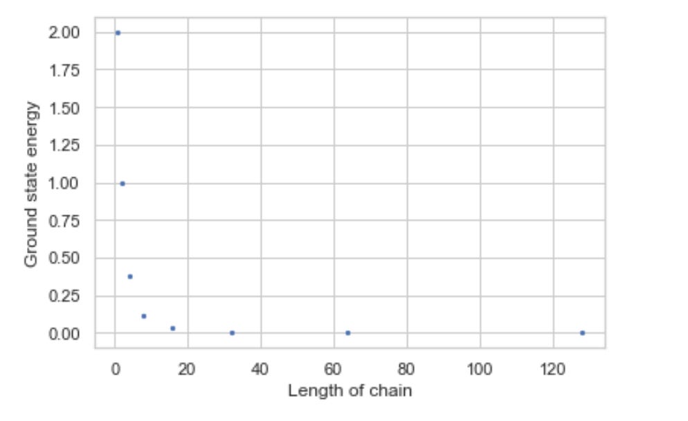
In the section below, I've put a code snippet on how I found the ground state energies.

from scipy.sparse import diags
from scipy.linalg import eig, block_diag
import seaborn as sns
sns.set() 
sns.set_style('whitegrid')

def ground_state_energy(size):
    
    diagonals = [[2] * size, [-1] * size, [-1] * size]
    H = diags(diagonals, [0, -1, 1]).toarray()

    evals, rvec = eig(H)
    return min(evals)

plt.scatter([2 ** i for i in range(8)], [ground_state_energy(2 ** i) for i in range(8)], s = 5)
plt.xlabel('Length of chain')
plt.ylabel('Ground state energy')