The Particle Comes Alive — Casual Physics Enjoyer

Sometimes small effects don’t matter. Sometimes they do. Maybe you lead a certain French nation but then the whispers of your people become a revolution. Maybe you are a meteorologist that forgot to take into account the wings of a butterfly. But it's hard to know when small things become a big deal. But the thermal physics of systems might give us a hint into when.

Brownian motion is an example of thermal effects causing a particle to drift. When you leave a particle alone, you expect it to stay still. But a particle is rarely alone. It may be in a gas, or in water, all of which have an affect on the particle through random effects.

And luckily for us, it's observable with a microscope, which makes it possible for independent scientists to study. I'm going to explain what Brownian motion is. Much more than you needed to know. Why it's counterintuitive, the math behind it, and when it breaks (which is when it gets interesting).

In 1827 Robert Brown looked at some pollen in water using a microscope. But he saw that the particles drifted, away from the centre, in a motion as if they were alive. This was strange because the water was stagnant, nor the pollen active in any way - and so it couldn't move because of those reasons. Furthermore, it didn't matter which type of pollen he used.

[The motions] resemble in a remarkable degree the less rapid motions of some of the simplest animalcules of infusions.

These motions were such as to satisfy me, after frequently repeated observation, that they arose neither from currents in the fluid, nor from its gradual evaporation, but belonged to the particle itself.
— Robert Brown, A brief Account of Microscopical Observations… (1828)

It was only later on that Jean Perrin drew these paths of such particles in water. He got something that looked like this.

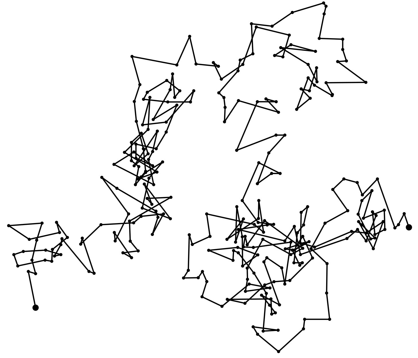
Jean Perrin's tracings of three colloidal particles, recorded at 30-second intervals. From Les Atomes (Paris: Félix Alcan, 1913). SVG rendering by ElioPrrl via [Wikimedia Commons](https://commons.wikimedia.org/wiki/File:PerrinPlot1.svg), CC0 / public domain.Wikimedia Commons, CC0 / public domain.*

But to the peoples of old, this drift was weird.

Water molecules are small and collisions are random. And because it’s random, the collisions against the pollen particle shouldn’t prefer any direction. Each collision placed a force on the particle. And since these forces averaged to zero, by symmetry, then the net force should be zero. Which means that the particle should not accelerate at all due to Newton's law of motion.

This was the classical view

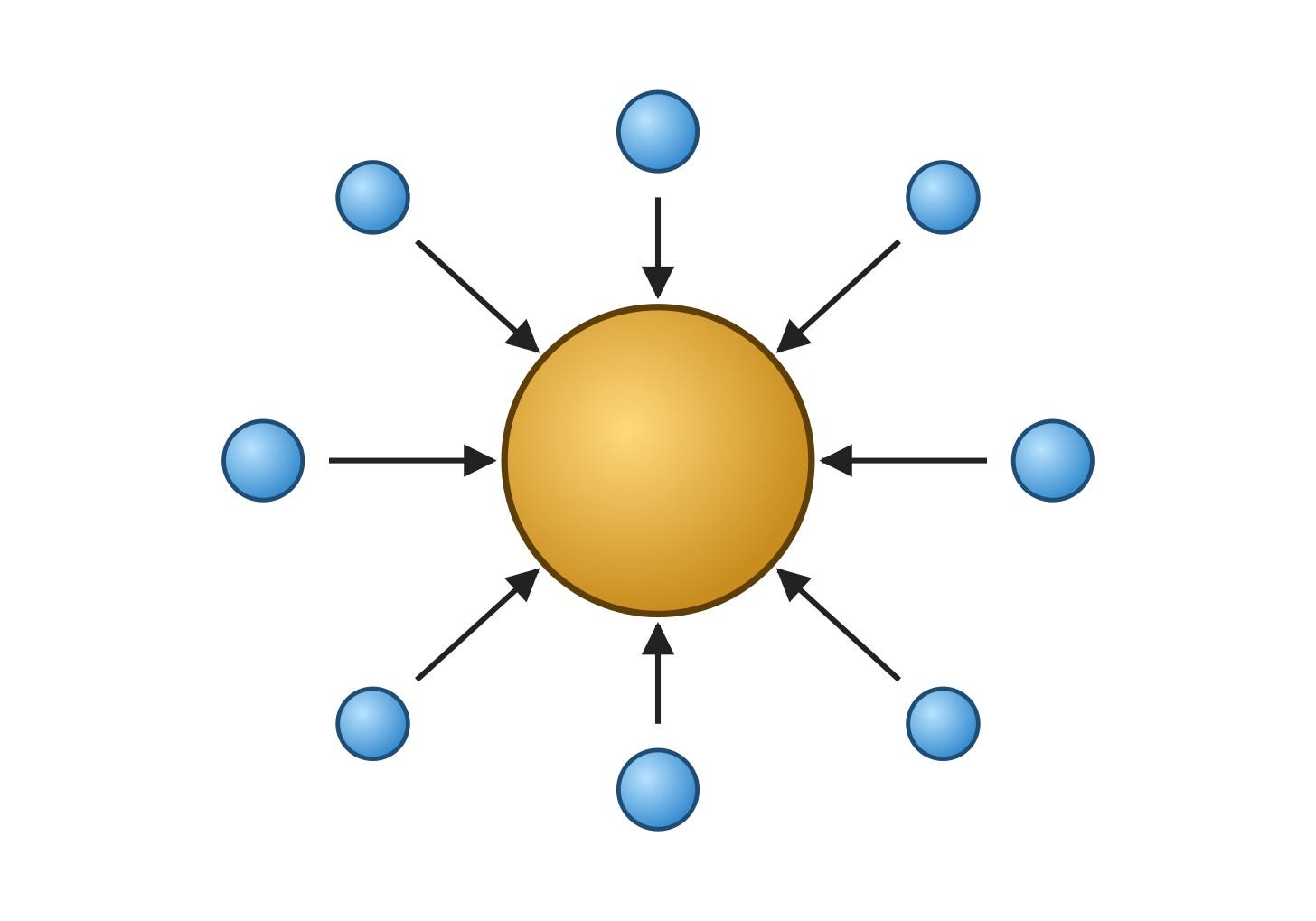
Water molecules hit the pollen particle from all sides. With collisions equally likely in every direction, the forces should cancel out and the particle should sit still.

By Newton's second law, we had

$$ F = ma $$

And if we take the average of the forces, then

\langle F \rangle = 0 = m \langle a \rangle

which means that the acceleration should also be zero. Which means that if the particle was stationary at the beginning, then it shouldn't move. But this didn't happen according to Brown's experiments!

The problem with the logic above is that the averaging is done too soon. What we are interested in is the distance from the start point, which is the magnitude of the displacement, given by

\text{distance} = \sqrt{x^2}

For now, forget about the square root - we can add that later. We want to compute the average squared displacement from the starting point.

In other words, if the displacement from a start point is x, then we want to compute

\langle x^2 \rangle

The reason why this is not zero is because the average of a squared random variable is not the same as the average of that variable, squared. ⟨a⟩ = 0 doesn't imply ⟨x⟩ = 0, nor does ⟨x⟩ = 0 imply ⟨x²⟩ = 0.

So how do we compute the average displacement ⟨x²⟩ in this scenario? Einstein originally came up with the derivation of what happens in 1905, but I find Langevin's approach made in 1908 more constructive. I will explain it here.

As usual, start with the forces.

If a pollen is in water the first force is the friction that the pollen has by travelling through water. This friction is given by a law discovered by Stokes, which says that the friction force is proportional to its speed. And the second term is this random kick felt by the molecules colliding with it. The force diagram is like this:

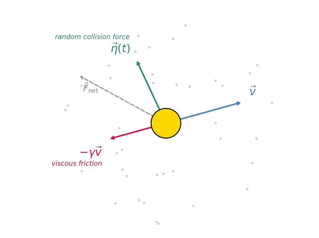
The pollen particle has a friction force -γ v against its motion and a random kick η(t) from the surrounding water molecules. The net force is F_net. In motion, it causes the particle to move like this:

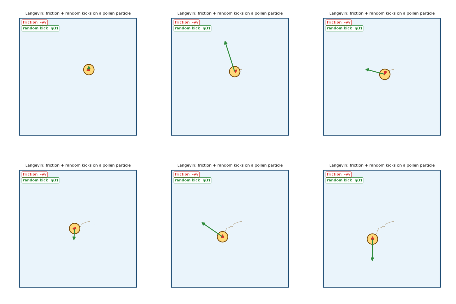
If we try to simulate the particles, it looks like they move away from the centre as a function of time. What is this function?

Since force is mass times acceleration, the equation of motion is the Langevin equation

m \frac{dv}{dt} = -\gamma v + \eta(t)

where m is the mass of the particle, v its velocity, γ a drag coefficient from the surrounding fluid, and η(t) is the random fluctuating force from the molecular collisions. The drag coefficient γ is given by Stokes law, which says that for a sphere of radius a moving slowly through a fluid of viscosity η_fluid, the drag force is proportional to its velocity:

\vec{F}_{\rm drag} = -\gamma \vec{v}, \qquad \gamma = 6 \pi\, \eta_{\rm fluid}\, a

The noise term has zero mean and is uncorrelated in time. Since it's selecting from random in all directions radially, the average is zero. In the notation below, the angled brackets mean 'average' over observations of η. So we have that

\langle \eta(t) \rangle = 0

For the second relation, we look at the correlation of the noise at two different points in time, t₁ and t₂. We assume the kicks are independent of each other — so the noise at one moment has nothing to do with the noise at another. But at the same moment, the noise has some variance K. Written as a case-by-case:

\langle \eta(t_1) \eta(t_2) \rangle = \begin{cases} K & \text{if } t_1 = t_2 \\ 0 & \text{if } t_1 \neq t_2 \end{cases}

The continuous-time version of this is ⟨η(t₁)η(t₂)⟩ = K δ(t₁ - t₂), where δ is the Dirac delta function. Right now, we've kept the distribution of this variable vague. All we know is that it has some variance K, and that it acts in random directions.

Ok, so how do we solve the Langevin equation? We want to compute the average of the squared displacement,

\langle x^2 \rangle

where we are taking an average over all of the paths of η(t). So visually, if we sample the brownian motion, measure x², then what is the average of that number?

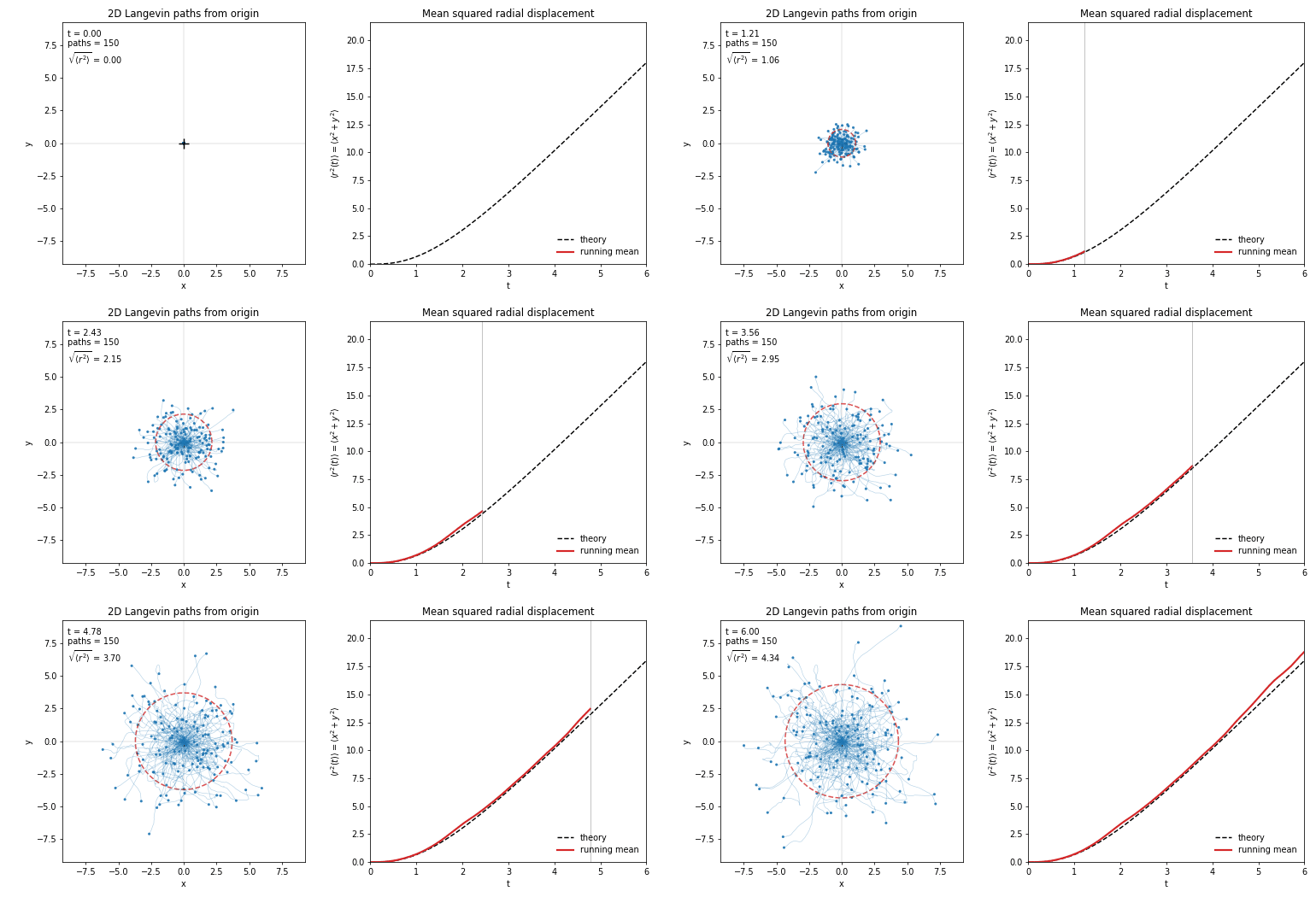
150 particles started at the origin spread radially under the 2D Langevin equation (left). The dashed red ring is the current RMS radius √⟨r²⟩. The right panel tracks ⟨r²(t)⟩ = ⟨x² + y²⟩, with the empirical mean (red) tracking the theoretical curve (dashed).

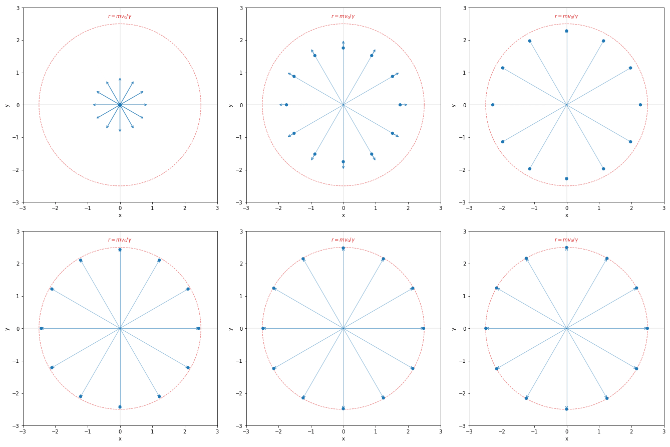
Modern treatments are quite complex. And I think Langevin's original argument to solve this is the best. Let's see what happens first if we try to solve the equation without the random force term.

m \frac{dv}{dt} = -\gamma v

This is something you learned to solve in high school. The solution is

v(t) = A\, e^{-\gamma t / m}

where A is a constant of integration. Imposing the initial condition v(0) = v₀ gives A = v₀, so

v(t) = v_0\, e^{-\gamma t / m}

Integrating once more, with x(0) = 0:

x(t) = \frac{m v_0}{\gamma}\left(1 - e^{-\gamma t / m}\right)

Now let's pretend for a moment that η is not a random variable but an ordinary function. Then we can solve the full differential equation exactly by variation of constants:

v(t) = v_0\, e^{-\gamma t / m} + \frac{1}{m}\int_0^t e^{-\gamma(t-s)/m}\, \eta(s)\, ds

This computes a single realization of η, but it doesn't directly tell us ⟨x²⟩. The following is Langevin's argument to compute the ⟨x²⟩. We have the force relation as above

m \frac{d^2 x}{dt^2} = -\gamma \frac{dx}{dt} + \eta(t)

Now we use a trick to rewrite the differential equation in a solvable form. Multiply both sides by x first.

m\, x \frac{d^2 x}{dt^2} = -\gamma\, x \frac{dx}{dt} + x\, \eta(t)

The benefit of multiplying by x is that you can rewrite the terms like this. (As a side note, you should remember the 'multiply by x' trick — it's useful in lots of other mechanics problems that require integrating something tricky).

x \frac{dx}{dt} = \frac{1}{2} \frac{d(x^2)}{dt}, \qquad x \frac{d^2 x}{dt^2} = \frac{d}{dt}\!\left(x \frac{dx}{dt}\right) - v^2

And when you substitute those in you get

m \frac{d}{dt}\!\left(x \frac{dx}{dt}\right) - m v^2 = -\frac{\gamma}{2} \frac{d(x^2)}{dt} + x\, \eta(t)

Now take the ensemble average ⟨·⟩ over realisations of η. We assume that the noise is uncorrelated with position, so that ⟨x η(t)⟩ = 0. The position x(t) only depends on η at earlier times, and η has no memory of itself, so its product with x averages to zero. We also assume the equipartition theorem: at thermal equilibrium, each quadratic degree of freedom carries ½ k_B T of energy on average.[^equipartition]

For a free particle in two dimensions, the kinetic energy ½m(vₓ² + v_y²) has two quadratic terms. Each gets ½ k_B T:

\langle \tfrac{1}{2} m v_x^2 \rangle + \langle \tfrac{1}{2} m v_y^2 \rangle = k_B T \quad\Longrightarrow\quad m \langle v^2 \rangle = 2 k_B T

Substituting this together with ⟨x η(t)⟩ = 0 into the equation from before:

m \frac{d}{dt}\!\left\langle x \frac{dx}{dt} \right\rangle - 2 k_B T = -\frac{\gamma}{2} \frac{d\langle x^2 \rangle}{dt}

Let z(t) ≡ ⟨x dx/dt⟩ = ½ d⟨x²⟩/dt. This gives us a differential equation for z:

m \frac{dz}{dt} + \gamma\, z = k_B T

Integrating this gives us

z(t) = \frac{k_B T}{\gamma} \left( 1 - e^{-\gamma t / m} \right)

And since z = ½ d⟨x²⟩ / dt, we can integrate this again to give us

\langle x^2(t) \rangle = \frac{2 k_B T}{\gamma} \left[ t - \frac{m}{\gamma} \left( 1 - e^{-\gamma t / m} \right) \right]

Ok, so what does this actually look like? You can see the displacement as a function of time here.

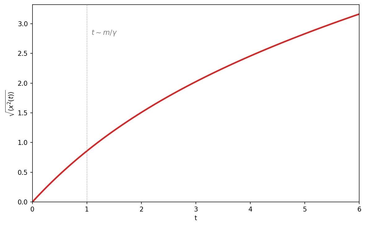
So, it starts curved, and then becomes straight. This has two regimes you can read off by hand, shown by the dotted line — when t is small, and when t is large. First let's see what happens when time is small. When γ t / m is small, we can Taylor-expand the exponential to cancel out some terms. The expansion is

e^{-u} = 1 - u + \tfrac{1}{2} u^2 - \tfrac{1}{6} u^3 + \dots

So with u = γ t / m,

1 - e^{-\gamma t / m} = \frac{\gamma t}{m} - \frac{1}{2}\!\left(\frac{\gamma t}{m}\right)^2 + \frac{1}{6}\!\left(\frac{\gamma t}{m}\right)^3 - \dots

Substituting into ⟨x²(t)⟩ = (2 k_B T / γ)[t - (m/γ)(1 - e⁻γ t / m)], the t and -(m/γ)(γ t / m) = -t cancel exactly. Then we get the leading term

\langle x^2(t) \rangle \approx \frac{2 k_B T}{\gamma}\left[t - \frac{m}{\gamma}\left(\frac{\gamma t}{m} - \frac{1}{2}\!\left(\frac{\gamma t}{m}\right)^2 + \dots\right)\right] = \frac{2 k_B T}{\gamma} \cdot \frac{m}{\gamma} \cdot \frac{1}{2}\!\left(\frac{\gamma t}{m}\right)^2 + \dots

After cancelling, we get the following. Note that it's dimensionally consistent, since both sides have units of distance squared.

\langle x^2 \rangle \approx \frac{k_B T}{m}\, t^2 = \langle v^2 \rangle\, t^2

This means that the average distance looks like linear motion, since

\text{distance} = \sqrt{\langle x^2 \rangle} = \sqrt{\langle v^2 \rangle}\, t

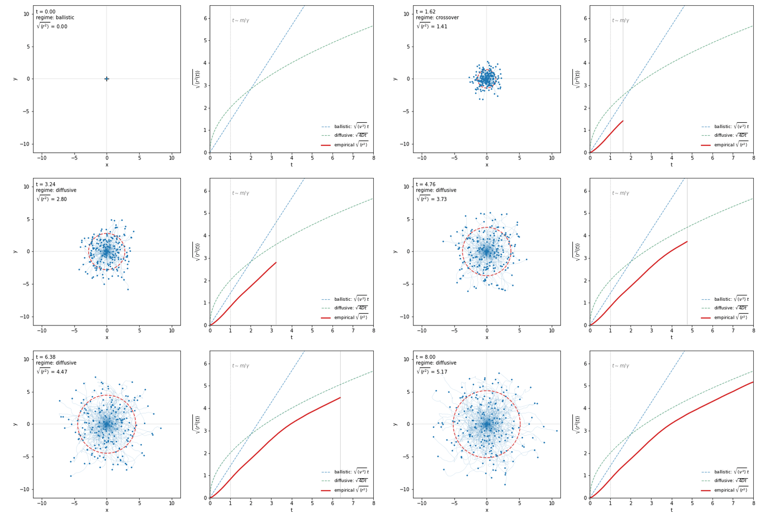
The particle just coasts ballistically at its velocity. But for long times the first term dominates, and the squared distance is proportional to time:

\langle x^2 \rangle \approx \frac{2 k_B T}{\gamma}\, t = 2 D t, \qquad D = \frac{k_B T}{\gamma}

Taking the square root,

\text{distance} = \sqrt{\langle x^2 \rangle} = \sqrt{2 D t}

You can see the two regimes in this radial animation here:

So how does this work in the wild? Does it show up in experiment? Here are 1-micron polystyrene spheres suspended in water, filmed through a microscope by Dr. Lejeune at the Institute for Advanced Physics:

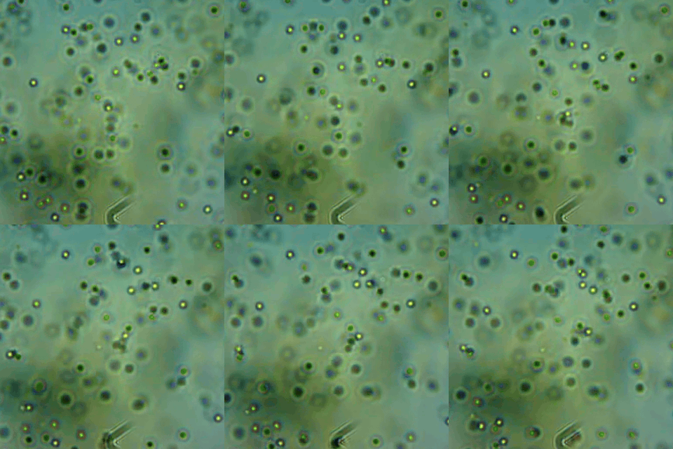
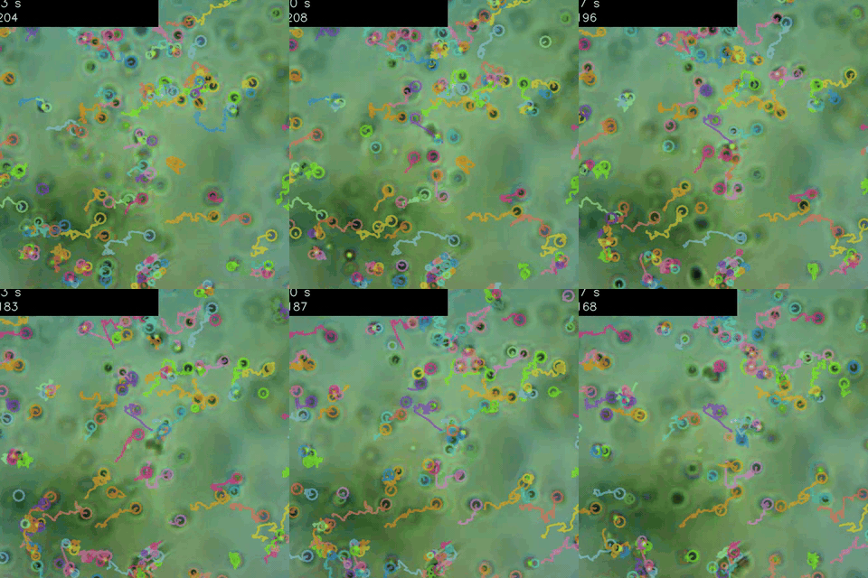
So does the relation hold in practice? I wrote a tracker (Laplacian-of-Gaussian blob detection per frame, then trackpy for linking, then a slope-1 MSD filter to keep only the diffusive particles) and ran it on Dr. Lejeune's video. The coloured circles below are the detected particles, with their recent trail showing the path each one has taken:

And so if we assume the system we're imaging is what the source says it is — 1 µm polystyrene spheres suspended in water at room temperature — we can compute the expected diffusion coefficient from the Stokes-Einstein relation:

D = \frac{k_B T}{6 \pi \eta a}

with

k_B = 1.38 × 10⁻²³ J/K (Boltzmann's constant)
T = 298 K (room temperature)
η = 1.0 × 10⁻³ Pa·s (dynamic viscosity of water at 20 °C)
a = 0.5 µm (radius of a 1 µm sphere)

Plugging in gives D_SE ≈ 0.44 µm²/s.

For 2D Brownian motion in the focal plane of the microscope, ⟨r²(t)⟩ = 4 D t, so the predicted RMS radius after t = 10 seconds is

\sqrt{\langle r^2 \rangle} = \sqrt{4 D t} \approx 4.2 \,\mu\text{m}

Comparing this to the data: I clipped each tracked trajectory to its first 10 seconds, subtracted the per-frame mean velocity (to remove fluid/stage drift in the sample), shifted each track to start at the origin, and overlaid all of them. The red dashed circle is the predicted √4Dt at t = 10 s.

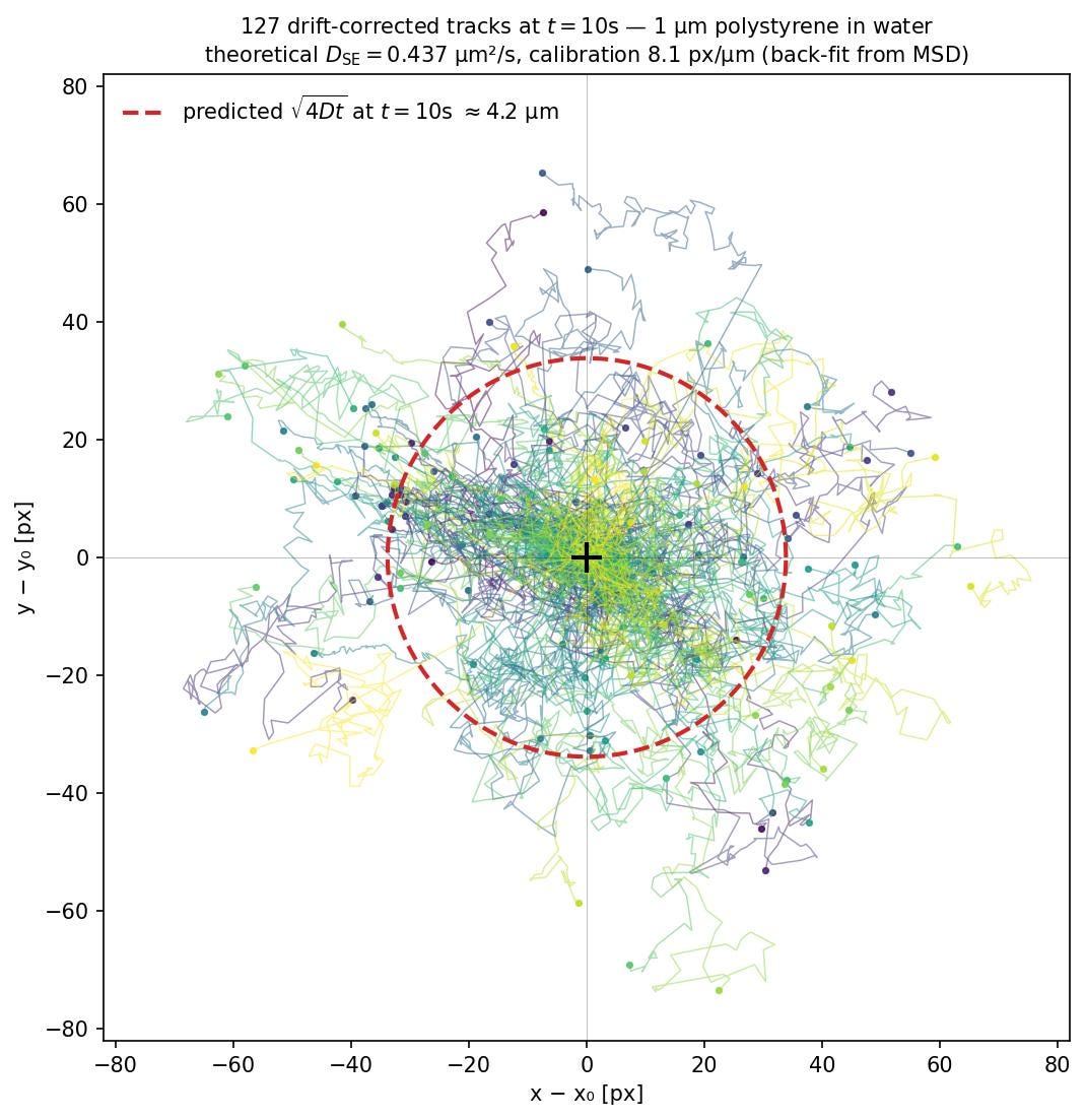
127 drift-corrected tracks from the video, each 10 seconds long and shifted to start at the origin. The dashed red ring is the prediction √4Dt ≈ 4.2 µm.

It's worth noting though that the tracking is quite janky since the footage isn't clear. This is why I want to get my own dataset, by filming milk fat globules like Michael de Podesta did in his post "Using a Microscope to observe Brownian motion" (Protons for Breakfast, March 2026), where he compares two cheap digital microscopes and films globules in diluted milk and flakes of graphite.

Now what next?

I've told you the story of Brownian motion, we can now question some key assumptions to probe for new physics. In the model, we assumed that the random impulses from the water molecules don't have memory. What if they did, and in what physical situations would this occur?

Indeed, there are many natural phenomena where the Brownian scaling laws don't apply. This is now known as 'anomalous diffusion' and seems to happen in the motion of live matter, active matter, and other non equilibrium processes. There is a lot of new physics out there and I hope to experiment with some non equilibrium processes and measure their diffusion rates in my homelab.

Footnotes

[^equipartition]: Why does each quadratic degree of freedom carry ½ k_B T? At equilibrium, the particle samples states with probability proportional to e⁻E / k_B T — the Boltzmann distribution. Suppose the energy contains a term that depends quadratically on some variable q, say E = ½α q². The average energy stored in that term, computed by integrating against the Boltzmann weight, is

\langle \tfrac{1}{2}\alpha q^2 \rangle = \frac{\int_{-\infty}^{\infty} \tfrac{1}{2}\alpha q^2\, e^{-\alpha q^2 / 2 k_B T}\, dq}{\int_{-\infty}^{\infty} e^{-\alpha q^2 / 2 k_B T}\, dq} = \tfrac{1}{2} k_B T

The α cancels — it doesn't matter how stiff the degree of freedom is, only that it's quadratic. So every velocity component, every position coordinate in a harmonic trap, every rotational mode gets ½ k_B T independently.

References

Brown, R. (1828). "A brief account of microscopical observations made in the months of June, July and August 1827, on the particles contained in the pollen of plants; and on the general existence of active molecules in organic and inorganic bodies." Philosophical Magazine, 4(21), 161–173.
Einstein, A. (1905). "Über die von der molekularkinetischen Theorie der Wärme geforderte Bewegung von in ruhenden Flüssigkeiten suspendierten Teilchen." Annalen der Physik, 17(8), 549–560. English translation in Investigations on the Theory of the Brownian Movement, ed. R. Fürth, trans. A. D. Cowper. Dover, 1956.
Langevin, P. (1908). "Sur la théorie du mouvement brownien." Comptes Rendus de l'Académie des Sciences (Paris), 146, 530–533. English translation: Lemons, D. S., & Gythiel, A. (1997). "Paul Langevin's 1908 paper 'On the Theory of Brownian Motion'." American Journal of Physics, 65(11), 1079–1081. PDF.
Klafter, J., Shlesinger, M. F., & Zumofen, G. (1996). "Beyond Brownian Motion." Physics Today, 49(2), 33.
Klafter, J., & Sokolov, I. M. (2005). "Anomalous Diffusion Spreads its Wings." Physics World, 18(8), 29.
Lejeune. (n.d.). Brownian Motion. Institute for Advanced Physics, Baton Rouge, LA. iapweb.org/brownian_motion.html. Microscope footage of 1-micron polystyrene spheres in water.
de Podesta, M. (2026). "Using a Microscope to observe Brownian motion." Protons for Breakfast, March 10. protonsforbreakfast.wordpress.com/2026/03/10/using-a-microscope-to-observe-brownian-motion. Comparison of two digital microscopes filming fat globules in diluted milk and graphite flakes.