Casual Physics Enjoyer

In my last post I described Freeman Dyson's toy model of a cell. Dyson made this model to capture qualitative aspects of autocatalysis, which is a process that involves products that speed up their own creation.

But I feel that his explanation of it in his origins of life book wasn't as clear as it could be. In some of the more mathematical parts, he tended to skip over some points which are disguised as easy, but are not straightforward. This is a shame because people who are rusty at math, or don't have mathematics in their formal training, are probably the most likely to find these kinds of models useful.

In this post, I wanted to fill those gaps with some interesting math on Markov chains, which I will explain in this post.

What is a reasonable toy model of a cell?

In the cell, we have N sites, where N is some ridiculously large number. These sites are meant to host monomers, which are simple chemical units. Each of these sites can be in one of three states. It can be empty, filled with an inactive monomer, or filled with an active monomer. For now, it doesn't matter too much what inactive versus active means. The word active is used because the more active monomers there are in the cell, the more likely it is that active monomers will spawn, and Dyson wanted a way to model this.

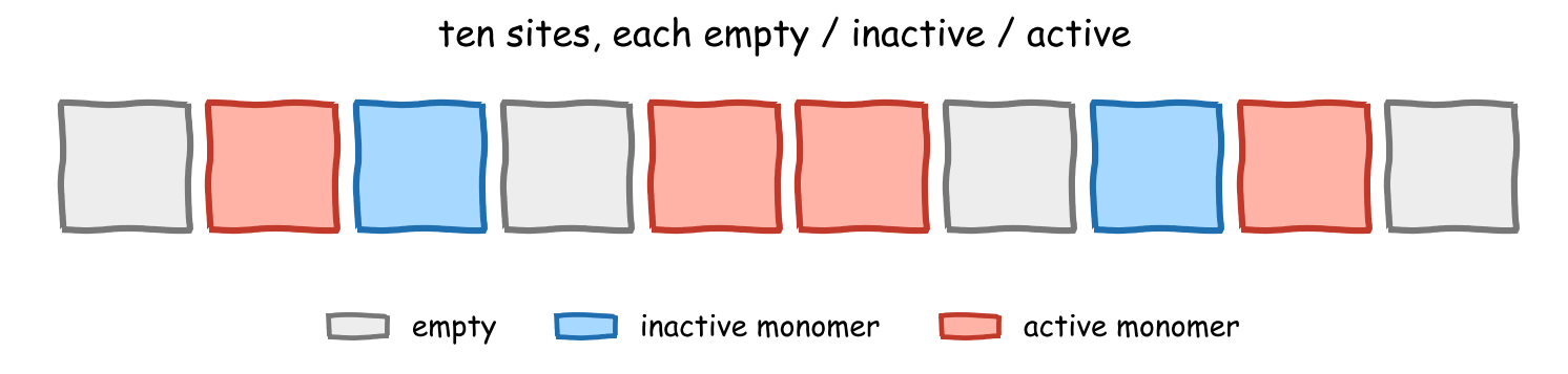
At any given time step, if a site is empty, then the probability that the site then gets an active monomer is ψ(x)p, where x is the fraction of sites that are already active, and ψ(x) is an increasing function. Dyson did it this so he could model autocatalysis, which means that the presence of something makes it more likely that this thing will be produced.

To be precise, x is just the fraction of all N sites that are currently active,

$$ x = \frac{\text{number of active sites}}{N}, $$

so x is a number between 0 and 1. The function ψ(x) is then any increasing function of that fraction, ψ: [0,1] → [0, ∞) with ψ'(x) > 0. The increasing part is the whole point: the more of the cell that is already active (larger x), the larger ψ(x), and so the more likely an empty site is to become active next. Dyson deliberately left the exact shape of ψ general — all that matters for the qualitative behaviour is that it goes up with x.

On the other hand, if a site is empty, there is also a chance that it gets an inactive monomer, where the probability of this is np, where n is the number of chemical species. Unlike the active monomers, having more inactive monomers doesn't increase the chances of inactive monomers occurring. The odds of an inactive monomer binding to a site stays fixed.

And if a site is filled by either an active or an inactive monomer, the probability of it becoming empty is qp. Dyson called this 'desorption'.

In all of the sentences above, the values p, q, and n are all constants. If we put this all together, we get a diagram that mathematicians use to reason about these kinds of systems.

This diagram has three nodes, each meant to represent a state, and each node has arrows showing the odds of transitioning to another node. In this diagram, it's worth noting that the probabilities leaving any node must add up to one. This is because if you're in a given state, you must go somewhere, so all the probabilities need to add up.

That means we can calculate the chance that an active monomer stays active, which would be 1 - pq, since the only way to leave the active state is to desorb. Similarly, the chance that an inactive monomer stays inactive is 1 - pq. We can also calculate the chance that an empty site stays empty: it's just one minus the chance that it becomes active minus the chance that it becomes inactive, which means that the chance an empty site stays empty is 1 - ψ(x)p - np.

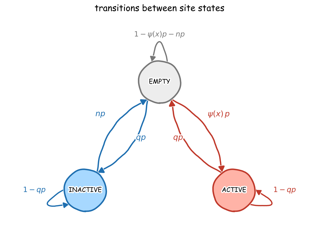
Interestingly, in this model, Dyson did not assign a probability that an active monomer would transform into an inactive monomer, or vice versa. For a site to have an active monomer changing to an inactive one, it must become empty first. If we were to add this transition probability, it would lead to some interesting math to do with loops in the chain, that I will explain in a future post.

So we now have this weird diagram, but how can we actually use it? In my last post, I didn't go into detail about how to think about these systems rigorously, so let's ask some dumb questions.

Suppose we had just 100 sites, all empty in the beginning. What happens next? Let's let the simulation run. The first thing you notice is that it seemingly settles to a stable proportion of inactive, active, and empty states. It wiggles around a bit, but the proportion quickly settles. The speed at which it settles is also an interesting question which I will not be covering here. The chart on the right shows the proportion of active, inactive and empty states as we move the model through time.

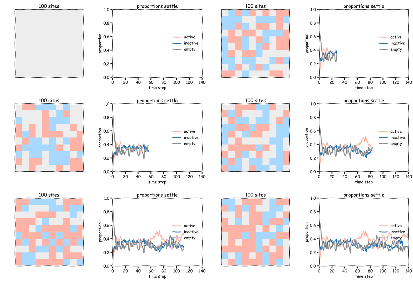
When we increase the number of sites, it becomes more obvious that the proportions 'settle' to some fixed value. You can see the lines on the bottom right settling to some fixed values, even though there is still some noise. Initially, we start from a place where all of the states are empty, but then it converges to some fixed values.

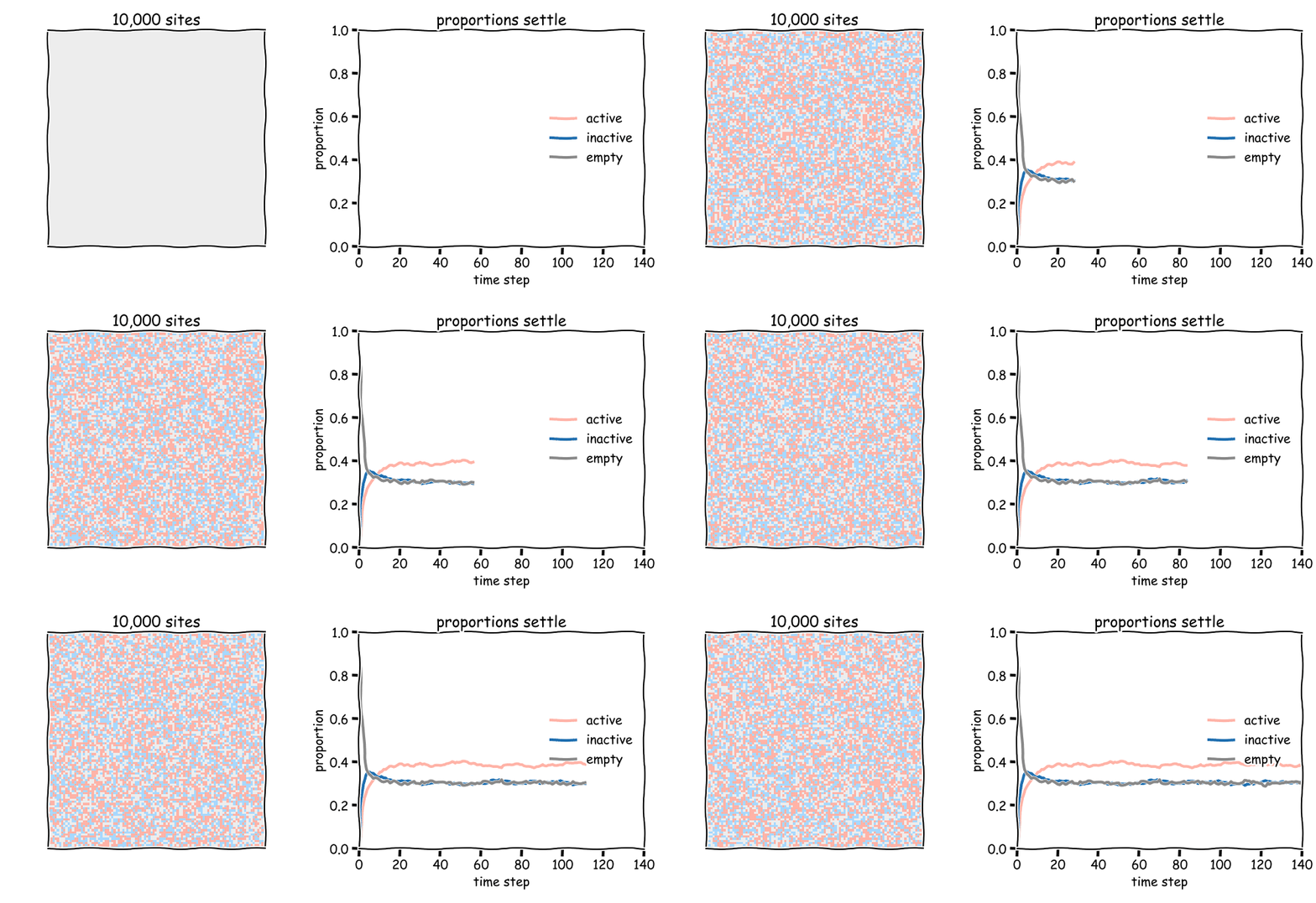
And this begs the question, what are these values as a function of ψ(x), p, q, and n? Can we model what they will be without having to do a simulation, and maybe find an analytic solution?

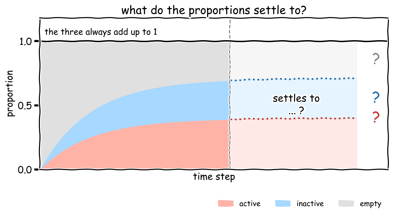
And also, how much do we expect the fractions to wiggle around these values? These are interesting questions because they are obvious, but the solution is unclear.

The Urn Model

To explore these questions, let's take a model of an urn to keep things simple. Suppose we have two urns, urns A and B. If we put a ball in urn A, there's a one-third chance of it staying there and a two-thirds chance of it going to urn B. And if we put a ball in urn B, there's a two-thirds chance of it staying there, but a one-third chance of it transferring to urn A.

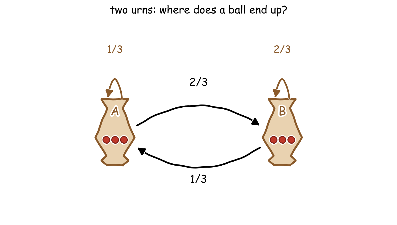
If we started with a hundred balls in A, what happens if we let the system run for a long time? Your rough guess might be that 1/3 of the balls end up in urn A, and 1/6 of the balls end up in urn B. And you'd be right. Well, let's try and simulate this as follows

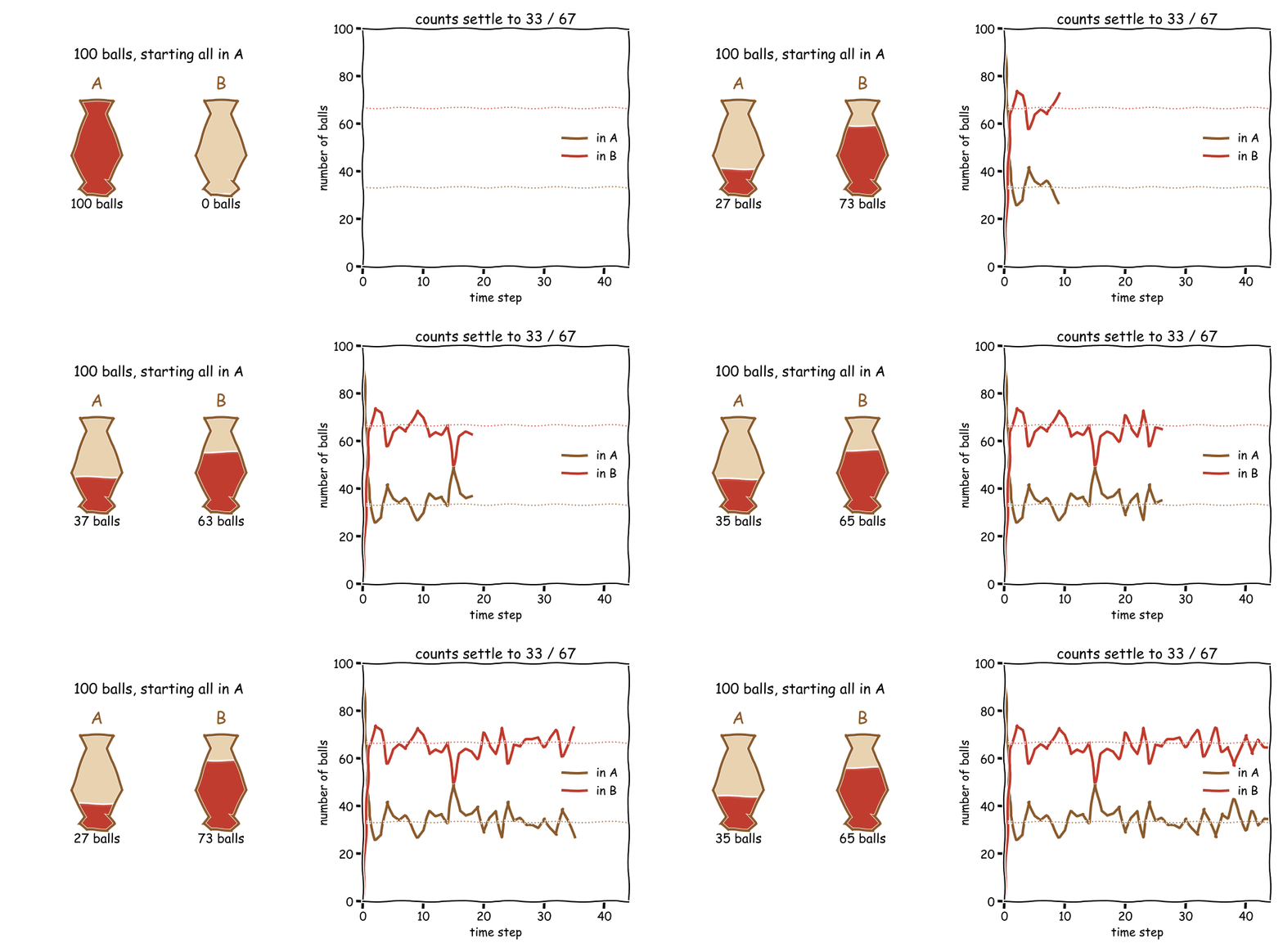
To solve this more rigorously, we can write out the system of two terms as a matrix. Suppose that p(A -> A) represents the odds of a ball going from urn A to urn A, p(A -> B) represents the odds of a ball going from urn A to B, and so on. Then we can construct something called a transition matrix.

$$ M = \begin{bmatrix} p(A\to A) & p(B\to A) \\ p(A\to B) & p(B\to B) \end{bmatrix} $$

There are some interesting properties of the matrix worth mentioning. It's not necessarily symmetric, but each column should add up to 1, because we are certain that if the ball is in urn A, then it MUST go to either A or B.

$$ p(A\to A) + p(A\to B) = 1, \qquad p(B\to A) + p(B\to B) = 1 $$

In our case, that is just 1/3 + 2/3 = 1 for each column. Also, since each entry is a probability, each entry must be between 0 and 1.

So what happens then to the distribution? If we start with 100 balls in A, we expect 1/3 of them to stay in A, and 2/3 of them to end up in B, then our allocation changes to 1/3 100 for A, and 2/3 100 for B on average. The way the math works out, this means that we can write down the expected distribution by multiplying the matrix with the initial distribution.

$$ \begin{bmatrix} \tfrac{1}{3} & \tfrac{1}{3} \\[4pt] \tfrac{2}{3} & \tfrac{2}{3} \end{bmatrix} \begin{bmatrix} 100 \\ 0 \end{bmatrix} \longrightarrow \begin{bmatrix} 33.3\ldots \\ 66.6\ldots \end{bmatrix} $$

So in general, we have the formula

$$ M \begin{bmatrix} A_t \\ B_t \end{bmatrix} = \begin{bmatrix} A_{t+1} \\ B_{t+1} \end{bmatrix} $$

In the example above, we used the example of a 100 balls to start with, but we can equally work in probability space too. Okay, so what distribution does it settle to? Well, if we look at the numbers, then this will settle when the numbers don't change, in other words, the distribution of balls reaches a steady state when

$$ \begin{bmatrix} A_t \\ B_t \end{bmatrix} = \begin{bmatrix} A_{t+1} \\ B_{t+1} \end{bmatrix} = M \begin{bmatrix} A_t \\ B_t \end{bmatrix} $$

Or in other words, we have that in a steady state, the transition matrix doesn't change the distribution.

$$ M \begin{bmatrix} A \\ B \end{bmatrix} = \begin{bmatrix} A \\ B \end{bmatrix} $$

And for those of you who have a math background, this looks familiar - the vector is an eigenvector, with eigenvalue 1! It is not always guaranteed that matrices have an eigenvector with eigenvalue 1, but the conditions I wrote above guarantee it; columns summing to one, and each entry being between 0 and 1. I'll write a proof of this in the appendix.

So let's try to solve the system of equations for the transition matrices in the urn model, and get A and B. So we have

$$ \begin{bmatrix} \tfrac{1}{3} & \tfrac{1}{3} \\[4pt] \tfrac{2}{3} & \tfrac{2}{3} \end{bmatrix} \begin{bmatrix} A \\ B \end{bmatrix} = \begin{bmatrix} A \\ B \end{bmatrix} $$

The solutions to this system are any vectors that are proportional to

$$ \begin{bmatrix} A \\ B \end{bmatrix} \propto \begin{bmatrix} 1 \\ 2 \end{bmatrix} $$

since the steady-state condition forces B = 2A. But we can always just normalise it and work in the space of probability distributions that the initial urns are filled with, so that

$$ A = \tfrac{1}{3}, \qquad B = \tfrac{2}{3} $$

which is exactly the 33/67 split we saw the simulation settle to. It's worth noting for later that the solutions could be anything proportional to the A B vector, but we can work in probability space by making sure that the elements of the vector add to one. This final settled distribution is called the steady state, and I will refer to it as such later on.

Extending this to the model of the cell

Let's apply this idea to Dyson's model of the cell above. We had the earlier diagram of the Markov chain here

If we represent each row / column as an empty, inactive, or active state, we then get the following transition matrix, in order of empty, inactive, and active probabilities.

$$ M = \begin{array}{c|ccc} & \text{Empty} & \text{Inactive} & \text{Active} \\ \hline \text{Empty} & 1-\psi(x)p-np & qp & qp \\ \text{Inactive} & np & 1-qp & 0 \\ \text{Active} & \psi(x)p & 0 & 1-qp \end{array} $$

As seen before, each column gives the chances of where a site in that state goes next. As before, each column adds up to one: for the empty column, (1 - ψ(x)p - np) + np + ψ(x)p = 1, and for the inactive and active columns, qp + (1 - qp) = 1.

And this means to find the steady state distribution, we need to figure out what distribution satisfies the equation we had earlier. Writing E, I, and A for the steady-state fractions of empty, inactive, and active sites, the equation we want to solve is

$$ \begin{bmatrix} 1-\psi(x)p-np & qp & qp \\ np & 1-qp & 0 \\ \psi(x)p & 0 & 1-qp \end{bmatrix} \begin{bmatrix} E \\ I \\ A \end{bmatrix} = \begin{bmatrix} E \\ I \\ A \end{bmatrix} $$

We can push the vector on the right side to the left, which just subtracts 1 from each diagonal entry, to get it like

$$ \begin{bmatrix} -\psi(x)p-np & qp & qp \\ np & -qp & 0 \\ \psi(x)p & 0 & -qp \end{bmatrix} \begin{bmatrix} E \\ I \\ A \end{bmatrix} = \begin{bmatrix} 0 \\ 0 \\ 0 \end{bmatrix} $$

And then fortunately for us, every entry on the left has a factor of p, and the right-hand side is zero, so we can cancel out the p:

$$ \begin{bmatrix} -\psi(x)-n & q & q \\ n & -q & 0 \\ \psi(x) & 0 & -q \end{bmatrix} \begin{bmatrix} E \\ I \\ A \end{bmatrix} = \begin{bmatrix} 0 \\ 0 \\ 0 \end{bmatrix} $$

Now, finding the solution to this is equivalent to finding the null space of this matrix (ie the set of vectors that map to zero), and the solution space is all vectors that are proportional to

$$ \begin{bmatrix} E \\ I \\ A \end{bmatrix} \propto \begin{bmatrix} q \\ n \\ \psi(x) \end{bmatrix} $$

And if we normalise this, we find that the E, I, A vector must be equal to

$$ \begin{bmatrix} E \\ I \\ A \end{bmatrix} = \begin{bmatrix} \dfrac{q}{q+n+\psi(x)} \\[10pt] \dfrac{n}{q+n+\psi(x)} \\[10pt] \dfrac{\psi(x)}{q+n+\psi(x)} \end{bmatrix} $$

But recall that x in this context was itself the proportion of states that were active, which means that the steady state of the Dyson cell model needs to fulfill the following condition where

$$ x = \frac{\psi(x)}{q + n + \psi(x)} $$

This is a self-consistency condition: x shows up on both sides, so the steady-state active fraction is wherever the curve g(x) = ψ(x)/(q + n + ψ(x)) crosses the line y = x.

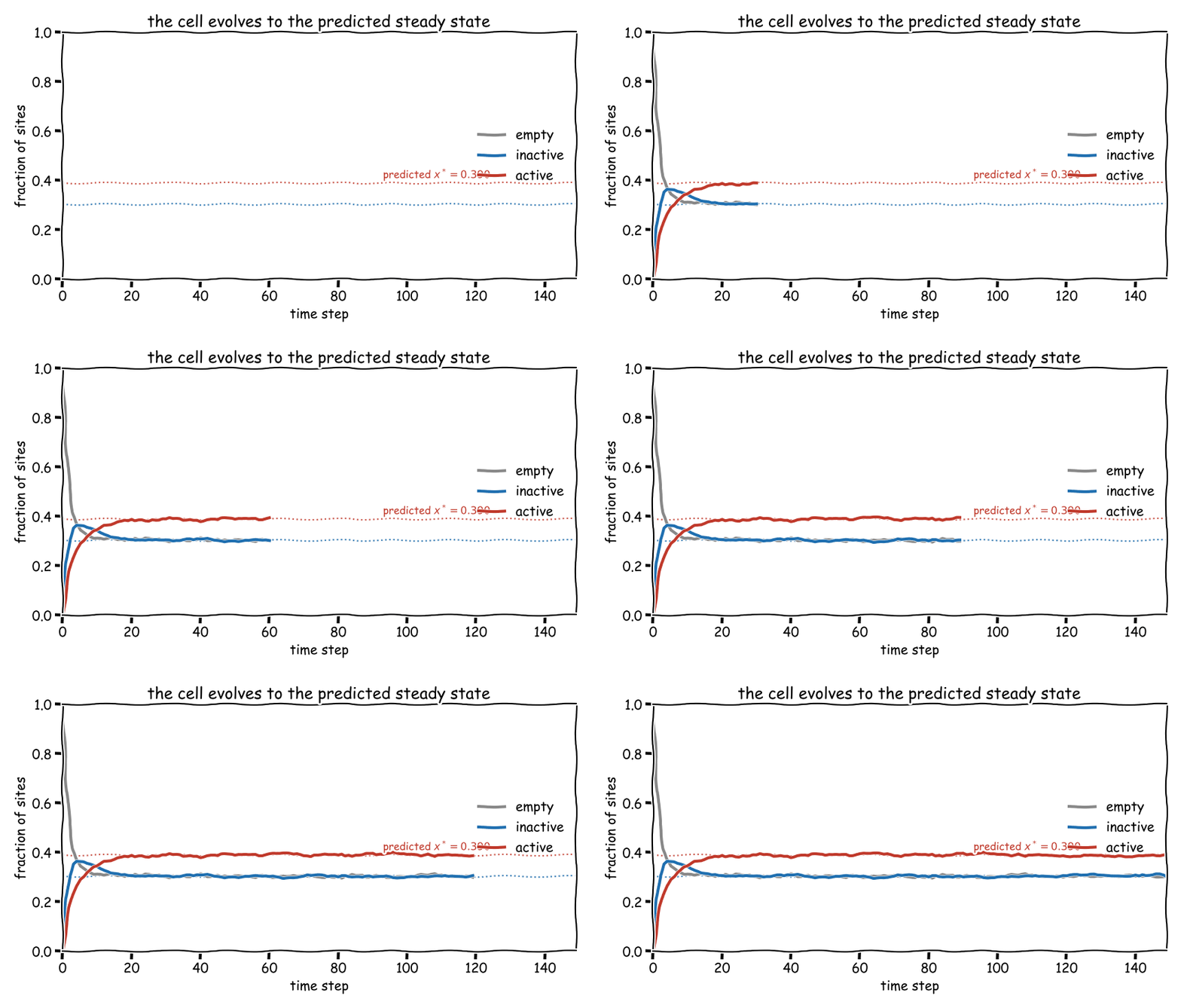
We can check that this is actually right. Taking the simple increasing function ψ(x) = 1 + 4x with p = 0.1, q = 2, and n = 2, the fixed point of g sits at x\* ≈ 0.390. If we then run the full agent-based simulation of the cell (20,000 sites, let it settle) and measure the proportions, they land right on top of the prediction:

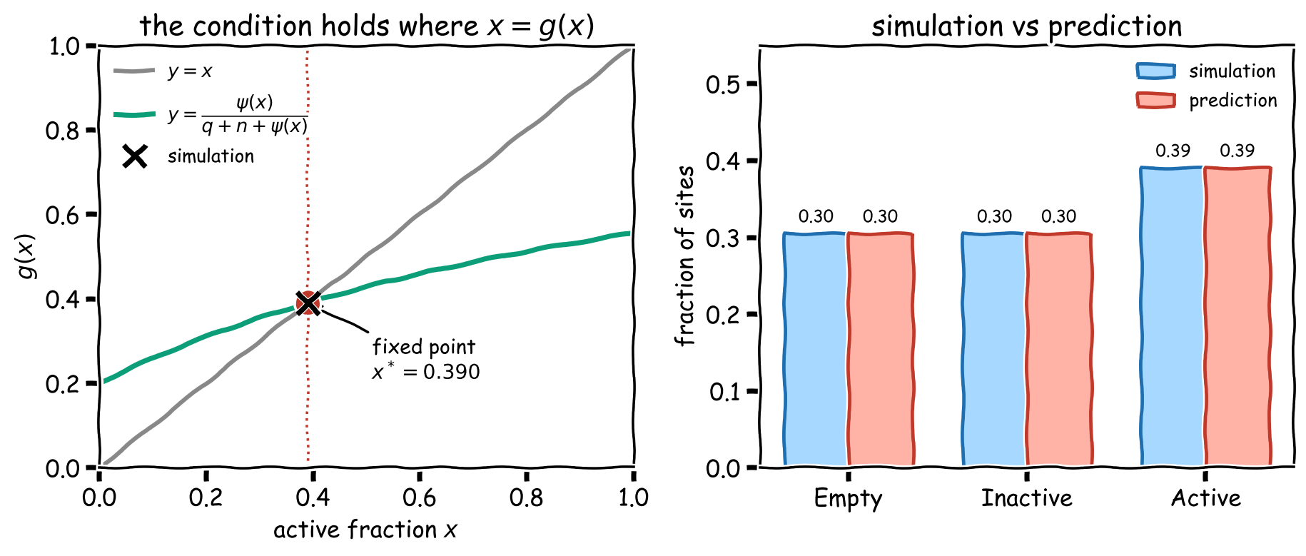
This is how it evolves over time — starting from an empty cell, the proportions climb and settle right onto the dashed prediction lines:

On the left, the simulation (the ×) sits exactly where y = x meets y = g(x); on the right, the simulated Empty / Inactive / Active fractions (0.305, 0.305, 0.390) match the analytic (q/(q + n + ψ(x\)), n/(q + n + ψ(x\)), ψ(x\)/(q + n + ψ(x\))) to three decimal places.

References

Dyson, Freeman J. Origins of Life. 2nd ed., Cambridge University Press, 1999.