Hydrogen and its Mysterious Energies
Exploring the subtle, puzzling quantum mechanics of the most basic atom there is.
The story of Hydrogen is an extraordinarily subtle and mysterious one. Since the dawn of time, physicists have used Hydrogen to test out broader physical theories that can be used to explain our universe. In particular, one important property that physicists like to look at is the range of energies Hydrogen atoms can absorb and emit. This energy structure of Hydrogen has revealed ample amounts of information used to formulate modern physics — from quantum mechanics to quantum field theory.
The way to do tests is surprisingly simple. Experimental physicists typically funnel energy into atomic gases using electricity and then see what comes out. What colours does it emit? What can we see? Hydrogen, in particular, is a great candidate for this probing since it's the simplest atom there is.
This process can reveal a lot about the natural structure of Hydrogen. Moreover, using this technique, we can discover a lot about the energy levels of Hydrogen — the levels and structure of the energies that Hydrogen atoms can retain. It turns out that the energy structure of Hydrogen is both surprising and complex, and it has motivated much of the physics we know today.
In particular, we now know that Hydrogen energy levels go up in discrete 'steps' instead of a smooth gradient. I'm going to cover why Hydrogen has a discrete set of possible energy levels, using the quantum mechanics of the 1930s.
In the next post, I will then explain the flaws of that theory and a mysterious effect called the Lamb shift that physicists could not explain with the rudimentary quantum mechanics of that decade. I will then talk about the Lamb shift and how it sparked the next flurry of physical inquiry — quantum electrodynamics. Throughout the way, I'll discuss the mathematical techniques used to usher in the quantum revolution of the 1950s.
The beginning — the orbital model of the electron
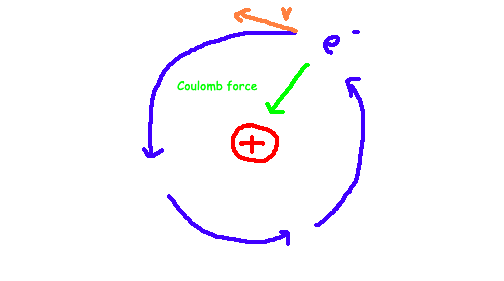
Let's start simple. The most basic model of the hydrogen atom in the 1900s involved a single electron orbiting one proton. We use gravity to explain the Moon's orbit around the Earth, and this model is very similar. In physics, for an orbit, we require two things. Firstly, there needs to be a central force pulling the two objects together. Secondly, the satellite object, both the Moon and the electron, needs to travel quickly enough to remain spinning around the central object and not get fully sucked in. But, on the other hand, it also can't go too fast so that it gets pulled away.
Let’s dig into the first part. A proton has a positive electric charge, and the electron has a negative electric charge. The electromagnetic force between these two particles is called the Coulomb force and says that when oppositely charged objects are closer together, the level of attraction between them increases. Before the advent of quantum mechanics, this model was not dissimilar to Newton's gravitational orbit model.
The shape of the Coulomb force and the gravitational force is precisely the same.

The equation on the right above allows us to compute the force between two charged particles. The q's in the equation represent the electric charge that each of the two particles has. The K in the equation is a universal constant, called Coulomb's constant. The term at the bottom is the radius. It is the distance by which the particles are separated. The force decays with the square of the separation. The gravitational force has the same shape, but instead of charge, we have mass. Instead of the Coulomb constant, we have Newton's gravitational constant.
The model of electrons orbiting around a central nucleus was in vogue in the early 1900s. At the time, people understood gravitation well — to keep something in orbit, there is a critical speed at which the satellite object needs to travel to make sure the central force does not entirely suck it in. Furthermore, the closer two objects are together, the stronger the attraction, so the orbiting satellite needs to go even faster. So, to ensure the constant orbit of the electron, we can even predict the speed at which the electron needs to whizz around the nucleus to stay in orbit; I'll explain this soon.
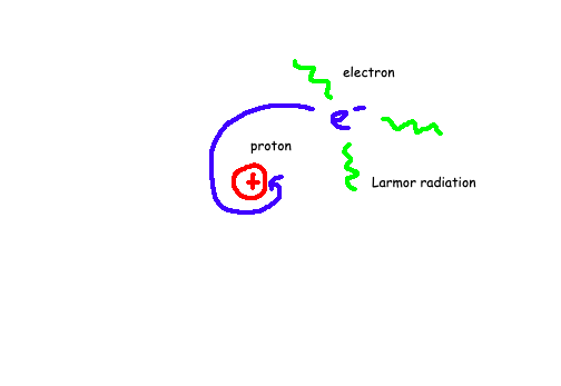
However, there were some problems with this orbital theory. First, there is an effect called the Larmor formula¹, discovered in 1897. The Larmor formula successfully predicts that charged particles under the influence of a force radiate electromagnetic energy in the process. In this case, since an electron orbiting a proton-nucleus is in a constant state of acceleration, it would mean that the Larmor effect would slowly drain energy from the electron. It is this precise effect that is used in antennae to transmit radio waves. The Larmor formula then suggests that the electron would rapidly collapse into the proton.
The fact that this doesn't occur means something fishy with the orbital model, which makes it qualitatively distinct from the Moon and Earth model.
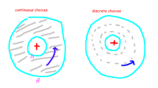
There is another thing wrong with the orbit model of the electron and proton. I mentioned previously that the model was analogous to the theory of gravity due to Newton. In Newtonian gravity, a satellite orbiting another object can be placed in a continuous set of distances from the central object, as long as it moves quickly enough. By continuous set, I mean that it is theoretically possible for the orbiting electron to live at any exact distance between A metres and B metres, to whatever decimal places and degree of precision you like. Any length would be valid as long as the satellite satisfies a certain velocity. In this case, A represents the minimum possible distance, and B is the maximum possible distance. Physicists can calculate these minimums and maximums from rudimentary orbital mechanics. Once you choose this, there is a corresponding speed that the object needs to remain in a stable orbit.
Below, we show the relationship between velocity and distance from the centre. For a circular orbit of an electron around a proton, we need this to hold.

The 'continuous allowed distances' is in contrast to a discrete set of distances. In discrete distances, orbits can only be chosen between particular 'steps' of lengths fixed from the centre. For example, a choice of either 1 metre, 1.1 metres, 1.4 metres and so on, is a discrete choice. It turns out that experimentally, an electron cannot travel within continuous distances from the proton. It is only allowed to live in a discrete set of distances. I'll explain how we've figured this out in the next section.
If there are a discrete set of distances, the electron can travel at only a discrete set of velocities. As a result, the energies that are allowed in the electron are also discrete. So, the energy levels of Hydrogen are locked in discrete steps.
As a side note, this notion of continuous range in classical gravity doesn't hold just for circular orbits. It also holds in orbits that are oval. In the case of gravitational orbit, a motion can orbit at any radius within the following range shown below. In the expression, e is the eccentricity of the orbit, which represents how different it is from a circle. There are also other inputs in this expression, including the masses of both the satellite object and the central object. The capital letter G represents Newton's gravitational constant.


The discrete energy spectrum
So, how did we figure out that electron orbits can only lie at discrete distances from the central proton? Well, the key was to look at the emission spectra of hydrogen gas. Emission spectra are the colours you get when you excite hydrogen gas with some electricity. It turns out there are only a discrete set of colours that appear, not a smooth, continuous spectrum! They are shown in the image below.

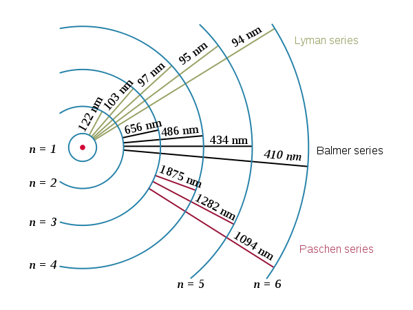
When a hydrogen atom gets excited with energy, the electron gains energy. Then, it emits light on the way back down. The fact that there are only a discrete set of colours emitted means that the electron can't have a set of continuous energies. It means that the different energies that an electron can only live in discrete levels. This is an amazing fact. At the small scale, we've now observed a very strong departure from the 'gravitational' model of electric charge. Instead of energy allowing to smoothly increase and decrease, we find that it becomes locked in discrete levels. In particular, the energies of each level are given by the formula.

The diagram below illustrates why this happens. When an electron is excited and shifts levels, it can only emit fixed quantities of energy, corresponding with fixed, discrete wavelengths of light. This is why we only see a small selection of colours in the picture above.
We've now explained what we've observed with the experiment. Now, it's time to get down to the model of why this happens. I'll first explain a fundamental quantum mechanical model used before Feynman's quantum electrodynamics but is still highly accurate. In the next post, I'll then explain this quantum mechanical model's weakness and talk about the Lamb shift and renormalisation.
Explaining the discrete energy spectrum with quantum mechanics
An atom is a small object. We know that nature doesn't obey the same laws present at larger scales on a small scale. So, it is naive for us to use a theory of gravity to explain the workings of an atom. Instead, we have to resort to quantum mechanics, a physical theory that begins to matter when we look at phenomena on the scale of the Plank distance.
I covered some basic ideas in quantum mechanics in an earlier blog post—Quantum mechanics models physical objects using probability distributions. For example, we model the electron's position — and other quantities like momentum — with a mathematical object called a wave function. The wave function is an abstract function that spits out a probability depending on where we look at the wave function.
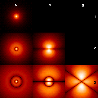
This means that if, say, an electron has a particular wave function that is 'large' in a given area, then if I observe the electron repeatedly in a series of experiments, I am likely to see the electron in that area more often.
To explain why we have discrete energy levels in Hydrogen, we have to figure out what the wave function of an electron near a proton looks like. We are now playing a different game to just using Newton's laws of gravitation. How do we even begin to figure out the form of this wave function, let alone the energy it contains?
This is where the famous Schrodinger equation comes in. The routine to figure out the form of the wave function is quite simple. First, we set the 'scene' by describing the environment of the electron. This scene translates into a particular equation. Once we solve it, it gives us a wave function from which we get a probability of a particle at every point in space.

The above equation is the Schrodinger equation in a qualitative form. This particular form of the equation is called the 'time independent equation'. This is because we only consider wavefunctions that don't change in time (those are more complex). The term on the left represents the energies that the wave function can have. In brackets, the first term with the funky looking symbols describes now the wave function changes in space.
The potential term is the interesting one. It is selected by the physicist to describe the 'environment' that the electron is placed in. It is merely a model. The potential that physicists inserted in the beginning took inspiration from the Coulomb force that we first discussed.

In all its glory, the complete form of the mathematical Schrodinger equation looks like this.

In the equation, the E symbol on the right-hand side is precisely the energy of a given wave function. So we need to solve this beast by finding a wave function that obeys this equation. There are also a few other conditions that a sensible wavefunction needs to satisfy.
Since wave functions describe probabilities, they can't just veer off to infinity and take infinitely large values. The wave function needs to be finite, and in some sense, needs to be contained in a relatively compact space.
Wavefunctions need to be mathematically 'continuous'; it is unnatural for them to be jagged in any way.
Once these conditions are in place, the rest is 'just math'. There are many different mathematical techniques that physicists use to solve this equation, including finding easy, 'mini solutions' that work and then combining them into a bigger solution. Another method is to use the symmetries of the space to restrict the set of possible solutions to ones we think are more compatible.
In particular, the kinds of 'mini solutions' used in a problem like this are called spherical harmonics.
Doing the math gives us two conclusions about the wave function solutions to this equation. These conclusions form the heart of why the energy levels of Hydrogen are discrete, and you may be surprised to find out they come from a line of pure mathematical reasoning.
The condition that a wave function needs to be finite leads to a set of mathematical equations that amazingly involve integer (whole number) values. These whole number solutions put stringent conditions on what the radius of an electron can be, which explains why the radius of the electron gets locked in at discrete steps. Hence, the energy also is locked in at discrete steps.
Energy is not the only value that needs to be locked into discrete steps. For example, the angular momentum, which is the circular analogue of standard momentum, also only can be observed in discrete steps! The discrete nature of angular momentum is what Niels Bohr hypothesised in his early model of the Hydrogen atom.
This method of making continuous quantities discrete is called quantisation. It is with this that we've explained the fascinating quantum nature of the hydrogen atom.
Wrap up
I hope you've learned something in this crash course on the quantum mechanics of Hydrogen! In the next post, I hope to cover Lamb shift and quantum electrodynamics. The Lamb shift is a peculiar anomaly at odds with the quantum theory I've explained here.
References
[1] Larmor J (1897). "LXIII.On the theory of the magnetic influence on spectra; and on the radiation from moving ions". Philosophical Magazine. 5. 44 (271): 503–512. doi:10.1080/14786449708621095. Formula is mentioned in the text on the last page.