Casual Physics Enjoyer

Racism in job and housing markets are the topic of ferocious debate in Malaysia. From my experience, debate on this topic is primarily fuelled by anecdotes and screenshots of messages on social media (please feel free to email me if I’ve missed out any substantial quantitative attempts that have been done already. These attempts should be openly posted on the internet, and not in paid-for academic journals).

There doesn’t seem to be much literature out there that actually quantifies this cost to the Malaysian economy. In this article, I will try to propose a model for a lower bound for the Ringgit cost of racial discrimination, at the job interview selection level. From this model, I hope to propose a break-even value that should be invested in polices that implement blind CV selection, or education to combat bias at the interview selection level.

Ideally, my hope is that this cost should be subject to further review and then submitted to the Malaysian government to put it in next year’s budget. Broadly, I would like to see more quantitative analysis by the Malaysian government in their policy making with regards to racial bias. I hope that this is a decent step in that direction.  

How should we define the economic cost of racial discrimination? I think a reasonable measure is to look at the productivity forgone from choosing poor candidates, at the expense of more productive ones, from racial bias at interview stage. Suppose we have a company, and they are chose a poor candidate since they are from preferred ethnic group A. They are likely to have also missed out on a good candidate from group B because they didn’t select them at the interview stage due to bias. If the candidate B was say MYR 1k more productive annually, then this would be the cost.

In this post, I put forward a first estimate that this sort of bias costs us around MYR 18 million annually. This is compared to an 'ideal scenario case' where employers correctly call superior candidates 60% of the time to interview, regardless of race. This does seem like a very large number and it shows the potential magnitude that the problem of discrimination is causing the country. I hope to find refinements to the model that will allows us to come closer to a more sensible definition.

Data

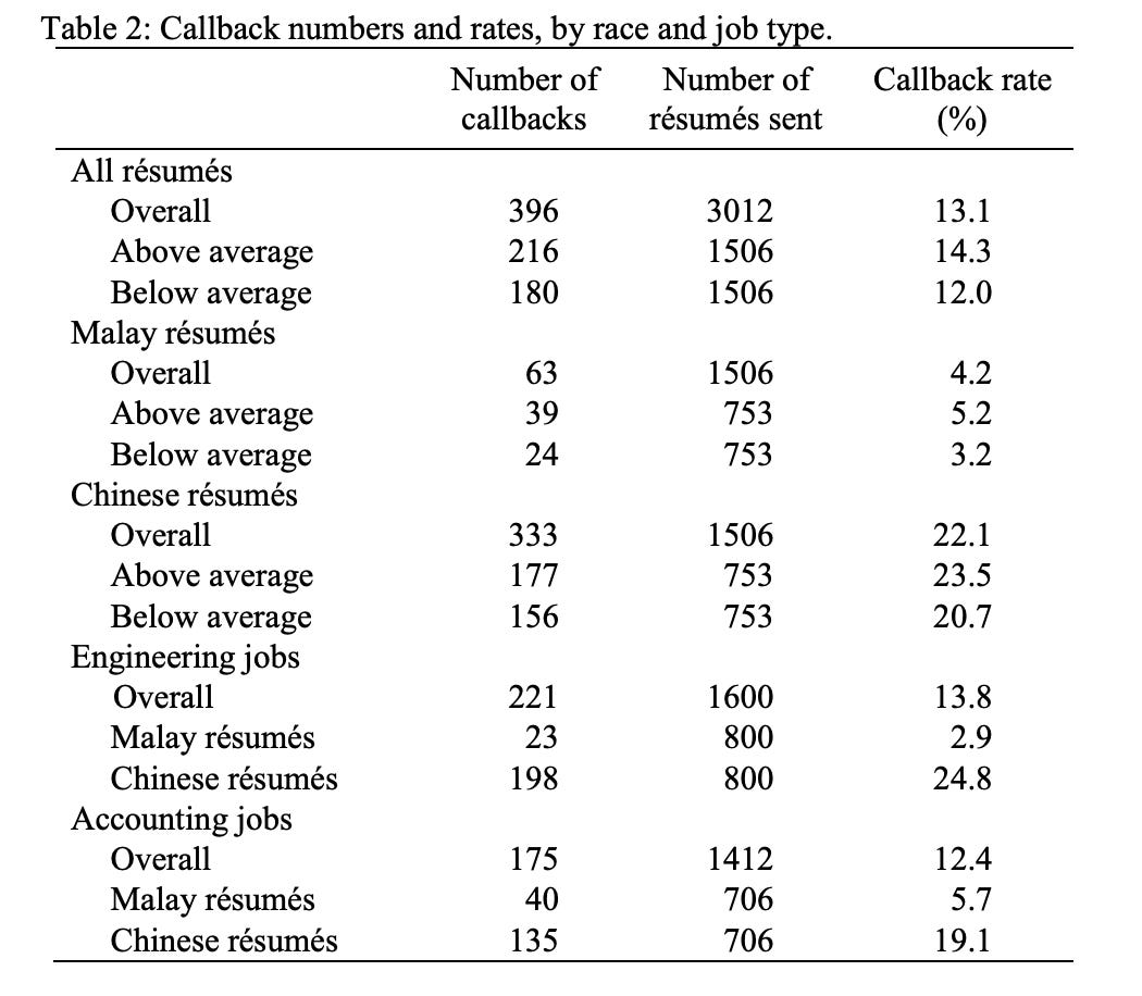
I will be working off of empirical data on a study by [1], as proxy inputs for this model. The inputs are call back rates as a function of race, and the quality of fake CVs generated by the authors of the paper. The table below shows the call back rate of resumes based on race and quality of their CV. A different resume was sent to a different company in this case.Note that the size of this sample is incredibly small, and the classification of above and below average resumes in the literature is muddy.

The Model

With this data, we will start to model the likelihood of selection based on race and its effect on productivity. Let’s start by assuming that each company in Malaysia receives 100 applications for each job posting. Due to constraints on interviewing, it is likely that each company brings 10 applicants to interview, and then chooses one applicant for the job. To model the success of an applicant, we will take the selection probability as

$$ P ( \text{Person from group j selected}) = \theta \times p_j $$

Where p_j is some preference probability, and theta is a filtering parameter that represents the probability of selection given that they get to interview. We will treat it as fixed.

Since we are studying the effect of racial prejudice between Malay and Chinese people, with two categories of skill at the screening level, we will model these 10 applicants as being chosen from a discrete distribution of people of 4 categories. I really want to emphasise that I am not taking a position here on what fields X in Malaysia bias ethnic groups Y. There is evidence of systemic racism in favour of ethnic Malays in many areas, and in favour of ethic Chinese in many other areas. For this reason I will label the groups A and B.

• Person from category A with an above average resume

• Person from category A with a below average resume

• Person from category B with an above average resume

• Person from category B. with a below average resume

We want to come up with an estimator for the number of skilled people from category A that were not selected at interview, and lost a job to a less skilled applicant who was. I am crap at probability and statistics, so it was easier to build a simulation. To do this, for each company, we will generate a sample of 100 applicants from a discrete distribution with parameters estimated from the table above, to represent the bias in selection. After this, we will then randomly select a set of 10 people from this sample of 100. The person who gets the job will be selected uniformly from this set of 10. If there is a person from group A, above average, that is not called in the set of interviewees, and it so happens that a person from group B, below average, is selected for a job, then we will tally this as one sample where there is a productivity loss. We will repeat this procedure several times. Ultimately we want to find

$$ \gamma = P(\text{not getting interviewed} | \text{Less skilled person from other group got the job} ) $$

How do we get the preference probabilities from the data above? Well, we aim to construct an estimator and then show that it is equal to the call-back statistics given in the data above. To break this problem down, let’s consider two people from A and B, each submitting a resume, and ignore the quality of the resume for now. For each potential candidate for interview, we model that the company will randomly select from A over B with some preference p, and then the probability that it selects a resume that the application was successful is given by some success rate theta, which is unknown. Let A be the event that a resume from person A was chosen, and similarly for B. In this case, we have that

$$ P( A = 1 )= \theta \times p, \quad P ( B = 1 ) = \theta \times ( 1 - p ) $$

Now, an unbiased estimator for p would be the following. Take the sums of the indicator function of A, then divide it by B. We find that rearranging, we get that an unbiased estimator is

$$ \hat{ p } = \frac{ \hat{A}}{ \hat{A} + \hat{B} }, \text{ where } \hat { A } = \sum _ i 1_ { A_ i } $$

Generalising further, if we have several groups A, B, C, D, then the preference probability would just be the following. I leave it as an exercise to show that this is unbiased. Hint: make sure you sum up independent variables when doing any division!

$$ \hat { p }_ A = \frac {\hat { A } } { \hat{ A } + \hat { B } + \hat { C } + \hat { D } } $$

So, the preference rate for a Malay person with an above average CV in this case, would be

$$ \frac{39}{39 + 24 + 156 + 177} $$

We the compare the difference of wrongly selected candidates to a baseline, where companies select above average candidates for interview regardless of race. This selection will be based on looking at the selection data for Malays. Our baseline is a preference for a higher than average CV of 60%, versus 40% for a below average CV.

The Simulation and Proposed Cost

We run a simulation of the model specified above, and then look at the probability of companies selecting a below average candidate from group B over an above average candidate from group A. We look at the difference between the baseline case, and the discriminatory case. Repeating this experiment 10 times over, we find that the mean difference of ‘poorly selected candidates’ between a discriminatory environment and a non-discriminatory one is around 60 hires per 10,000 companies.

To model this, we will assert that a high output person can produce an output of MYR 1000 higher than their counterpart with a ‘below average CV’. Now, why do I think that a reasonable estimate? , the standard deviation of income in 2021 across all of Malaysia was MYR 1800, which implies a similar deviation in productivity annually. In addition, the average productivity for a worker was MYR 22k annually.

Assuming we have around 800000 job postings per quarter (the most recent estimate by the Malaysian Central Bank), this puts the total cost of racial discrimination at MYR 18 million annually.

Code used for the simulation

companies = 10000
candidates = 10 
total = 39 + 24 + 177 + 156
fair_selection  = .5 * (39 + 177) / total 
fair_selection_null  = .5 * (24 + 156) / total 

classes = {
    'A_above' : 0, 
    'B_above' : 1, 
    'A_below' : 2, 
    'B_below' : 3, 
}

probabilities = {
    0 : 39 / total, 
    1 : 177 / total,
    2 : 24 / total,
    3 : 156 / total,
}

elements = probabilities.keys()

p = probabilities.values()
p_fair = fair_probabilities.values()

biased_selection = np.zeros(companies)
good_selection = np.zeros(companies)
A_in_interview = np.zeros(companies)
B_below_average_selected = np.zeros(companies)

selected_biased = np.zeros(100)
selected_non_biased = np.zeros(100)

for j in range(10):
    
    print(j)
    
    for i in range(companies): 

        applicants = np.random.choice(list(elements), 10000, p=list(p))
        interviewees = np.random.choice(applicants, 10)  # get a list of prefferential 
        A_in_interview[i] = np.sign(np.isin(interviewees, [2]).sum())

        biased_selection[i] = np.random.choice(applicants, 1)[0]
        B_below_average_selected[i] = int(biased_selection[i] == 3)

    df = pd.DataFrame([A_in_interview, B_below_average_selected]).T
    output = df.loc[( df[0] ==1 ) & ( df[1] ==1 )].sum()[0]
    selected_biased[j] = output 
    
    for i in range(companies): 

        applicants = np.random.choice(list(elements), 10000, p=[.5 * 0.6, .5 * 0.6, 0.5 * .4, .5 * .4])
        interviewees = np.random.choice(applicants, 10)  # get a list of prefferential 
        A_in_interview[i] = np.sign(np.isin(interviewees, [2]).sum())

        biased_selection[i] = np.random.choice(applicants, 1)[0]
        B_below_average_selected[i] = int(biased_selection[i] == 3)

    df = pd.DataFrame([A_in_interview, B_below_average_selected]).T
    output = df.loc[( df[0] ==1 ) & ( df[1] ==1 )].sum()[0]
    selected_non_biased[j] = output

    
## calculate produce 
output

References

[1] Lee, Hwok-Aun, and Muhammed Abdul Khalid. "Discrimination of high degrees: race and graduate hiring in Malaysia." Journal of the Asia Pacific Economy 21.1 (2016): 53-76.