What's A Good Theory Of Biology?
Science aims to produce theories. I want to do this for biology. But to do that, I need to describe what a good theory would look like. A good theory of biology probably involves finding simple patterns in systems with large numbers of meaningful variables.
In this essay I will describe what that means and how I am trying to do that.
I believe this work is relatively neglected. When I studied math, reducing the complexity of biologically inspired systems wasn’t taught in depth. It’s an important question, and physicists are well suited to work on it. After all, it was Schrödinger who made the first solid attempt in his essay ‘What is Life?’.
Conversely, I don’t see many biologists working on this stuff either. Most are working on micro scale things like proteomics or connectomics, without looking at dimensional reduction on the macro scale!
There was a flurry of statistical mechanics in biology work done by Zwanzig, but it’s died out, bar an essay by Pankaj Mehta: Theory is dead. Long live theory! For a 21st century statistical physics of life. Since we have much stronger computers, I think this is worth revisiting.
Biology has a lot of meaningful variables
A theory should predict how things change when the experimenter changes something: If we change parameter X, we should know how a set of variables Y, Z and so on, change.
It’s hard to make a theory of biology because there are many meaningful variables. So it’s hard to find which variable X is important, or how it works as part of the larger system.
In physics, the many particles in a gas or metal system also constitute many variables. But perturbing a single particle wouldn’t have a meaningful change on the system beyond just noise. In biology however, it’s different. Altering a single gene in a cell could have a big effect on the organism downstream.
John Hopfield talks about this in “Physics, computation, and why biology looks so different.”:
Why does biology look so different? As a physical system, it is just another example of dynamical broken symmetry. But what sets it apart from other such systems is its complexity—its meaningful information content. Meaningful information, as distinct from noise entropy, can be recognized by the fact that changing a meaningful bit alters the macroscopic behavior of the system.
In biology, the meaningful bits that encode macroscopic broken symmetry are stored in DNA as a single long string of nucleic acids. Changing even one of these can produce a large-scale effect on an organism’s behavior or viability. Physics is not used to dealing with systems whose macroscopic dynamic properties are so strongly influenced by single molecular-level events, nor with systems containing such vast amounts of significant broken-symmetry information.
So how do we solve this problem problem of ‘many Xs can cause many Ys’?
We want both a language, and intuition, about how to find patterns in big complicated systems. One way is doing a computer simulation of a big system of equations, and then seeing what 'lower dimensional’ ideas come out of it.
For example, suppose I describe a big, dynamic system of variables. Is there a ‘aggregate variable’ that describes most of the meaningful phenomena that is going on? Is there self correcting behaviour? Is there equilibrium behaviour? Is there something weird and unexpected? Do somehow all of the variables end up behaving the same?
The Lotka-Volterra Equations
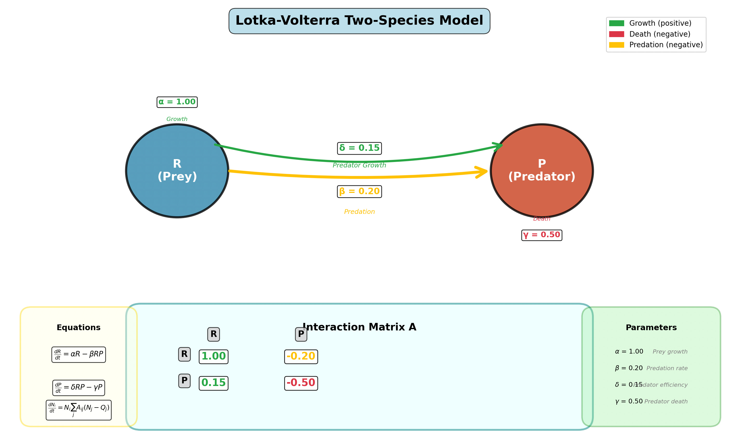
One way to start is just to pick a cool looking dynamical system and see what happens when we make it much more complex. From ecology, there’s an obvious candidate - the Lotka-Volterra (LV) equations. The LV equations are meant to model the number of species in an ecosystem, by writing down differential equations that model the relationship between predator and prey.
If we represent R as the number of prey, like a plant, we model it to have a natural growth rate alpha, which is damped by the number of predators feeding on it. With the predators P, we model them they to have a natural death rate, and make them grow according to how much prey there is in the system. The differential equation is
$$ \begin{align} \frac{dR}{dt} &= \alpha R - \beta R P \\ \frac{dP}{dt} &= \delta R P - \gamma P \end{align} $$
I simulated this in python. The prey and predator population change throughout time is shown below on the left hand side. The solid lines show how the predators evolve under different parameters, and the dashed lines show the prey. In the middle chart, I plot the number of predators as a function of prey.
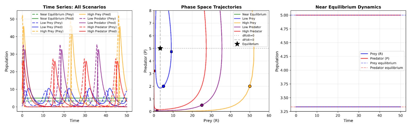
Depending on the parameters, the numbers of predators and prey either oscillate, or just stay at an equilibrium level and stay constant. This is interesting because its not immediately obvious that we get oscillatory behaviour, unless you think really hard. The phase space diagram shows the number of predators as a function of prey.
The LV equations it’s also pretty general too as a system. We don’t just have to describe predator and prey - this system is pretty much general enough to encode any behaviours that involve ‘interactions of sustenance’.
Extending It To High Dimensions
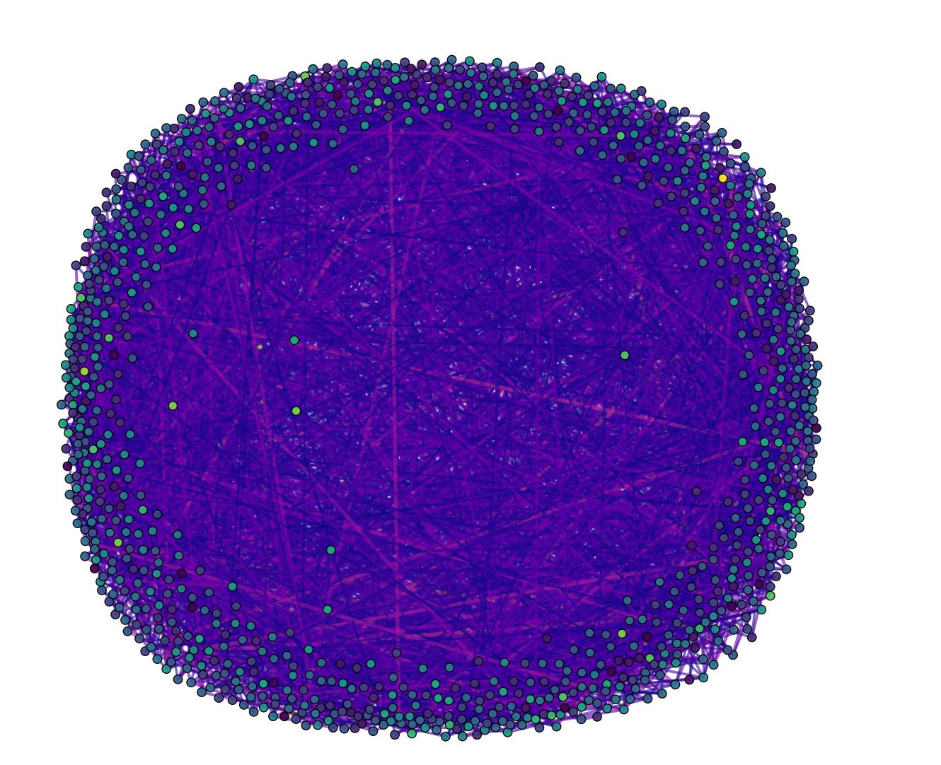
Now we’ve covered the simple case, lets do the more realistic scenario where we have thousands of variables. A system with thousands of species, and relationships between them will look like this web.
Mathematically, we can write this system as a big Lotka-Volterra system. In the equation below, population N_j evolves according to some function of the other species.
$$ \frac{\mathrm{d} N_j}{\mathrm{d} t} = \sum_{k=1}^{S} a_{jk}\, N_j\, \bigl(N_k - Q_k\bigr), $$
where N_j is the number of species, a_jk are the entries of an antisymmetric interaction matrix, and Q_k are the equilibrium populations. This antisymmetric matrix is nothing more than just the predator and prey parameters, but in the big case, and contain all the information about how each species interacts. For the sharp-eyed among you I’m glossing over the fact that equilibria actually may not exist, which I will aim to explain in a later post.
I set the number of species to simulate as 1000. Then, I chose random values from a normal distribution to generate the values a_jk, and used a numerical method called Runge-Kutta order 4 to find out how the species evolved in time.
Then I selected a random species to study, and varied the number that it initially started at. This is what came out. The first graph shows what happens when the initial number of species 53 is small. The second is when it starts as high. The last is when its really high.
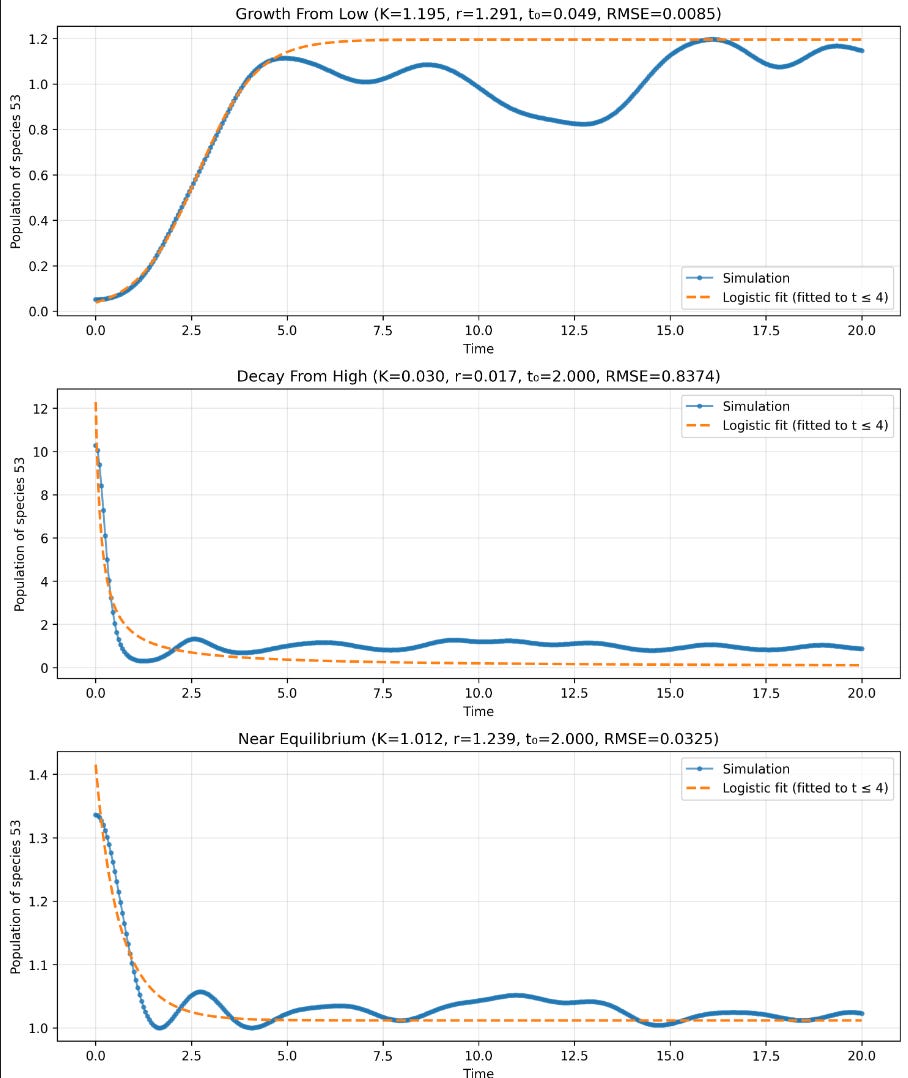
No matter where the species starts off, the number always comes back to its equilibrium value in a short amount of time. But what’s cool is how it gets there - is follows the shape of a logistic curve. The logistic curve is described by this equation.
$$ N(t) = \frac{K}{1 + \left(\frac{K}{N_0} - 1\right) e^{-r t}} $$
It’s not obvious that the Lotka-Volterra equations would out something like this. We initially started out with a system of equations with thousands of variables (encoded in the matrix a_ij), and yet if you choose any species, you get behaviour that looks pretty simple - a logistic curve, along with some noise. Zwanzig took this further and got something that looks even closer to the simulation, with something called a ‘hereditary kernel’.
I simulated this below, and you can see that it captures the characteristic ‘overshoot’ and ‘undershoot’ in the beginning.
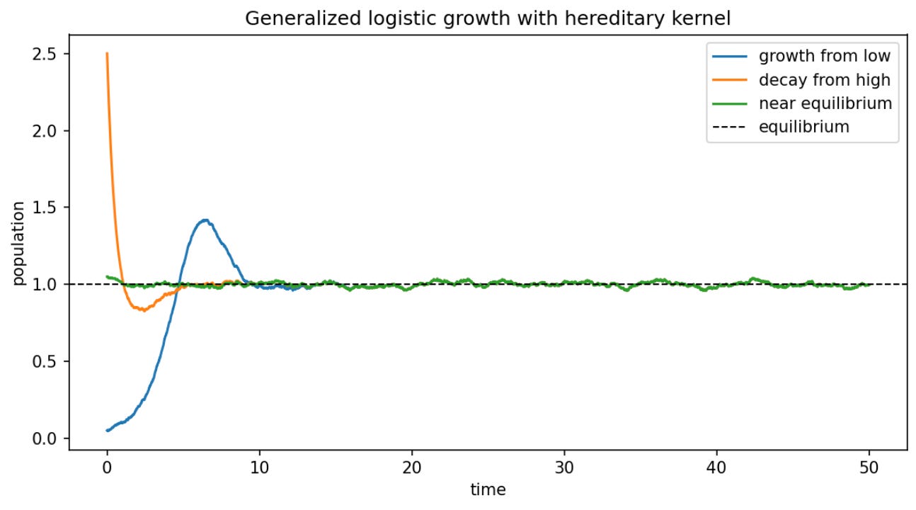
So in a system of many variables, we have characteristic behaviour that we can extract, that is encoded in the parameters r and K. Now, we can try to perturb this system of many parameters, and see how the dynamics change.
What happens when we keep the matrix the same, but slowly scale it up. When the matrix is scaled to zero, there are no interactions between the different species, so the population remains constant (in the top left graph). However, the more you scale up the matrix, the faster each species goes to equilibrium.
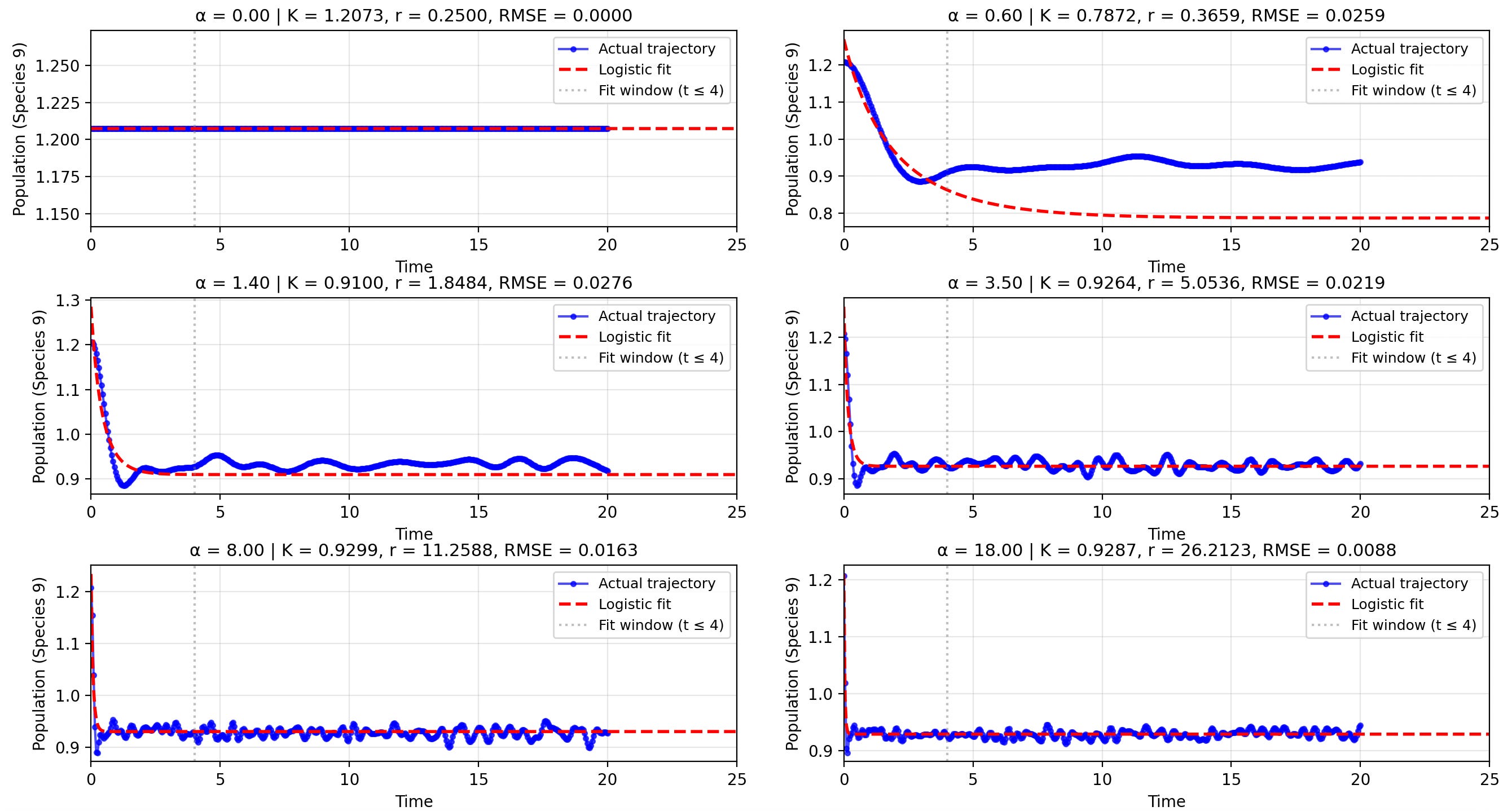
Increase scaling increases the speed to equilibrium. It also reduces the variance around the equilibrium, since populations are more reactive to one another when they get out of wack. This is cool because in this case, we have a bunch of parameters that we can reduce to a single parameter. The interpretation is that stronger couplings between different species leads to faster convergence to equilibrium.
For this species, I fitted a logistic regression to each trial, and got out the parameter r and K. When you increase the size, of the interaction matrix, the values of K and r change like the graphs below.
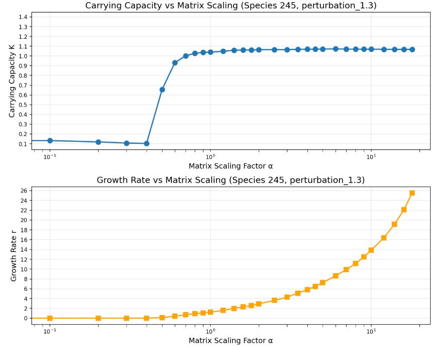
In general, I want to see how perturbing the parameters in the LV equations change the dynamics. In this example, I’ve scaled it. But there many different things you could do to the matrix a_ij. For example
Remove the equilibrium constraints
Rotate this high dimensional matrix
Increase the variance amongst the couplings
Zero out a bunch of the entries according to some random pattern.
Chemical Kinetics Equations
The Lotka-Volterra equations are pretty general already. But, they are unable to describe other kinds of dynamics that we care about in biology. We also care about chemical kinetics, which aims to describe reaction rates of different substances with differential equations. Chemical kinetics equations look like this
The competitive reaction-diffusion system below models embryonic development, based on concepts from Waddington’s work on how cells make fate decisions during development. We have three chemical A, B, and C and two processes P and Q which compete for the chemical B.
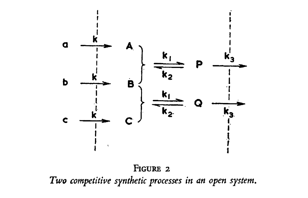
In this example, we have competing dynamics. The processes P and Q are like two chefs competing for these ingredients
chef P needs A + B
chef Q needs B + C
Both recipes need ingredient B . Moreover, once you’ve made some Recipe P, it helps you make more Recipe P faster (its are self catalytic). Same with recipe Q. The differential equation this system is
$$ \begin{aligned} \frac{dA}{dt} &= k(a - A) - k_1 P \cdot AB + k_2 P^2 \\ \frac{dB}{dt} &= k(b - B) - k_1 P \cdot AB + k_2 P^2 - k_1 Q \cdot BC + k_2 Q^2 \\ \frac{dC}{dt} &= k(c - C) - k_1 Q \cdot BC + k_2 Q^2 \\ \frac{dP}{dt} &= k_1 P \cdot AB - k_2 P^2 - k_3 P \\ \frac{dQ}{dt} &= k_1 Q \cdot BC - k_2 Q^2 - k_3 Q \end{aligned} $$
I then simulated this, and you also get logistic type behaviour, as well as some cool non linear behaviour.
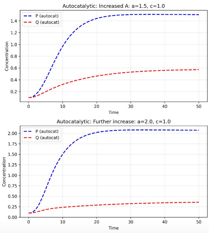
The equivalent high dimensional model would be something like this, which I think is new. I want to look at this in high dimensions as well.
$$ \frac{\mathrm{d} N_j}{\mathrm{d} t} = \sum_{j, k=1}^{S} a_{ijk} N _ k N _ k + \sum _ j b _ { i j } N _ j $$
Is This Actually Helpful For Humans
A good theory of biology would help us reason better about complex systems. I think this would only be valuable if there were immediate, killer applications that we could test it on. Here are some things that I think would be cool
Predator prey models
Inactivation mechanics for viruses in humidity
Plant microbiome for growing things
How cells synthesise proteins
How resources are allocated in embryo morphogensis
For example, if you look at how epidemiologists traditionally look at humidity and temperature, would would build a network of a bunch of causal factors. Presumably, we could turn this into a very big system of equations, and then try to measure how much things change when one variable is perturbed, or if things stay the same.
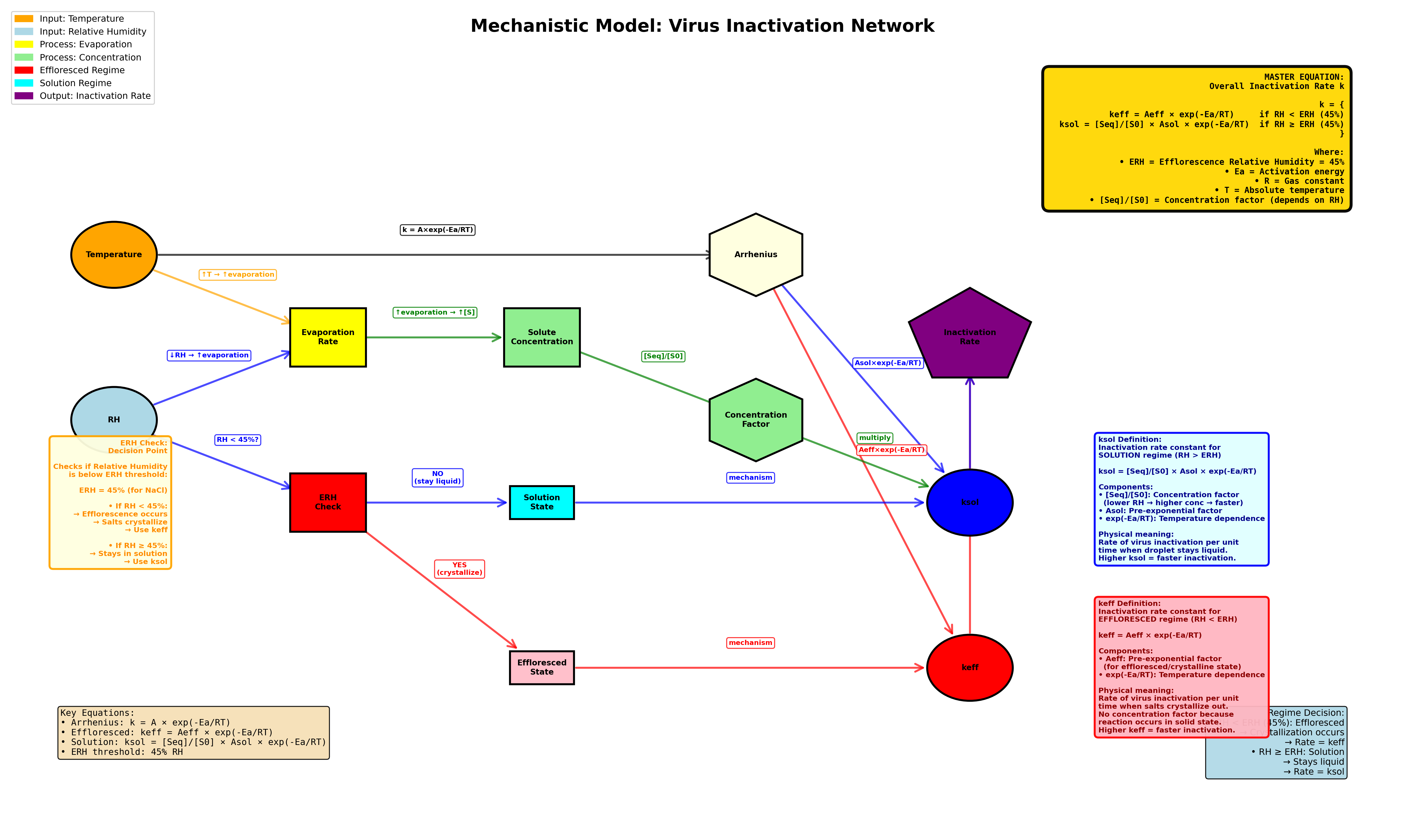
Everything I’ve said in this post is vague. But I think that’s a sign that there is something to do here. For my next investigation, I’ll be looking more at the Lotka-Volterra equations under relaxed constraints. If you are interested in looking at this stuff as well, get in touch!
Acknowledgements
Thank you to David Jordan at Living Physics for extensive discussion and ideas. All mistakes are mine.
References
Zwanzig, R. (1972). Generalized Verhulst laws for population growth. Proceedings of the National Academy of Sciences of the United States of America, 69(10), 3038-3040.
Mehta, Pankaj. “Theory is dead. Long live theory! For a 21st century statistical physics of life.” (2025)
Hopfield, John J. “Physics, computation, and why biology looks so different.” Journal of Theoretical Biology 171.1 (1994): 53-60.
Schrödinger, Erwin. What is Life? Cambridge University Press, 1944.
Statistical Mechanics Methods
Zwanzig, Robert. “Nonlinear generalized Langevin equations.” Journal of Statistical Physics 9.3 (1973): 215-220.