Slippage in Automated Market Makers
A First Look at AMM protocols in DeFi
I wanted to take a leisurely detour from my usual world of theoretical physics. In this post, I will talk about order books and their increasingly popular DeFi alternative — Automated Market Makers. In particular, I’ll discuss constant product market makers and go into a bit of the math of price slippage.
Order Books
Exchanges are open places where market participants can buy and sell objects. On an exchange, an order book is a traditional mechanism that large groups of people can use to decide prices to buy and sell things to one another. An order book consists of a bid side, and an ask side. The bid side consists of the sizes and prices that market participants are willing a buy specific security for. The offer side consists of sizes and prices market participants are willing to sell a security for.
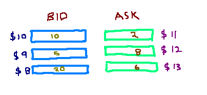
In the example below, we have an order book of oranges. The ‘bid’ side is shown on the stack on the right-hand side. The available sizes are 10, 5 and 20 at prices of $10, $9 and $8, respectively. This means that if I held oranges and I wanted to sell them, I could theoretically sell at most ten at $10 since there are willing buyers for that size. Conversely, there will also be a range of ask sizes and ask prices representing the size and price of market participants willing to sell an object.
I’ve drawn out this example in the picture below. If I was desperate to buy this object, I could choose to intercept the best bid at $10, and buy 2 oranges at $11 from the ask level.
Automated Market Makers
Whilst they are among the most popular methods for price discovery, order books are not the only mechanism to exchange objects for a price. There are plenty of different ways market participants can price things — each having its advantages and disadvantages for market participants and the economy in general.
This post will explore other types of exchange mechanisms in decentralised finance. One of these ways is where the price of two objects is determined by relative supply in a pool of available tokens. The exchange of these objects happens between two classes of market participants called ‘liquidity providers’ and ‘liquidity takers’. Liquidity providers contribute tokens to a pool of tokens, and liquidity takers swap tokens for other tokens from this book. These pools are called liquidity pools, and the mechanisms to price these objects fall under a large class of pricing protocols called ‘automated market makers’. I illustrate a liquidity provider adding tokens to a pool in the diagram below.
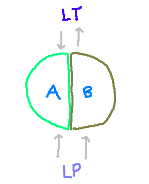
The LP contributes specific quantities of token A and token B to the liquidity pool. The LT then swaps token A for token B in a particular ratio (the price) that is determined by a pricing protocol. This protocol is typically dubbed an ‘automated market maker’. In exchange for the several risks that the LP takes on for committing liquidity, a transaction fee is also embedded into the price. In a future post, I’ll elaborate on these risks further.
Automated market makers apply formulas to price swaps based on the number of tokens (liquidity) they have. There are several types of procedures, ranging in popularity. There is a wealth of literature on each scheme’s effects, advantages, and disadvantages. These are still subjects of active research. Suppose that a and b represent the number of two different tokens — token A and token B, available on a liquidity pool. The three most popular protocols are
Constant product market makers — where a x b = k = constant.
Constant sum market makers — where a + b = k = constant.
Hybrid Market Makers — where some other function of a and b is held constant.
Constant Product Market Makers
It is called an automated market maker because the price given to liquidity takers is already pre-determined. This section will describe a particular type of AMM called a ‘constant product market maker’. A constant product market maker has the constraint that the product of the number of tokens A and B must be constant. Here is an example of how a constant product market maker works. Suppose that we have a market maker that starts with 30 of token A and 10 of token B. This means that the total product of tokens remains constant at 300.

Now, what is the “price” of a token on this exchange? To the first order, A’s price is just the ratio of how many B tokens you need to exchange for it. In this case, the price of token A in terms of token B would be

This constraint creates a price curve, where we can plot out the two prices of each asset based on how many assets there are in the pool at a given time. This is also commonly called a bonding curve. The x-axis shows the amount of A and the y axis shows the amount of B.
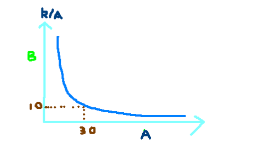
We can also convert this into price space by scaling it down. If you think about it, having more of token A in the liquidity pool will decrease its price relative to B. The above curve holds true in terms of the number of contracts. However, in terms of another contract in price space, we can do the following.

On the right-hand side, we have two terms in the product. The first is the price of token A in terms of another token C. The second term in the product is the price of token B relative to the token C. If contract C was, say, the US dollar, and assuming that this value stays constant, we have that the prices of each token in USD multiplied together are constant. In this case, the tokens’ prices have an inverse relationship to one another. This looks similar to the curve above.

The above is only accurate to the first order. What happens when we have someone that wants to trade with the AMM? In trading with the AMM, traders modify the values available in the liquidity pool. Well, the product of 300 must remain constant. Suppose that a trader wants to buy 5 of token A. How many tokens of B will they receive in return? Well, if this transaction takes place, we have the following equation. In this case, L_a and L_b represent the initial liquidity of tokens A and B. delta_a represents the change in the number of token A in the liquidity pool, and delta_b represents the change in the number of token B in the liquidity pool.

Supposed that our liquidity taker wanted to sell some of token A in exchange of token B. The advertised price of this transaction would be L_b / L_a. However, in transacting, the liquidity taker actually is changing the ratios of the tokens in the liquidity pool, resulting in a slightly different price. The realised price is based on the ratio using these updated quantities. Suppose that the liquidity taker wanted to sell some of token A to the AMM in return for token B. This means that, solving for delta_b, we would find that they need to receive

This means that the realised price of the transaction would be

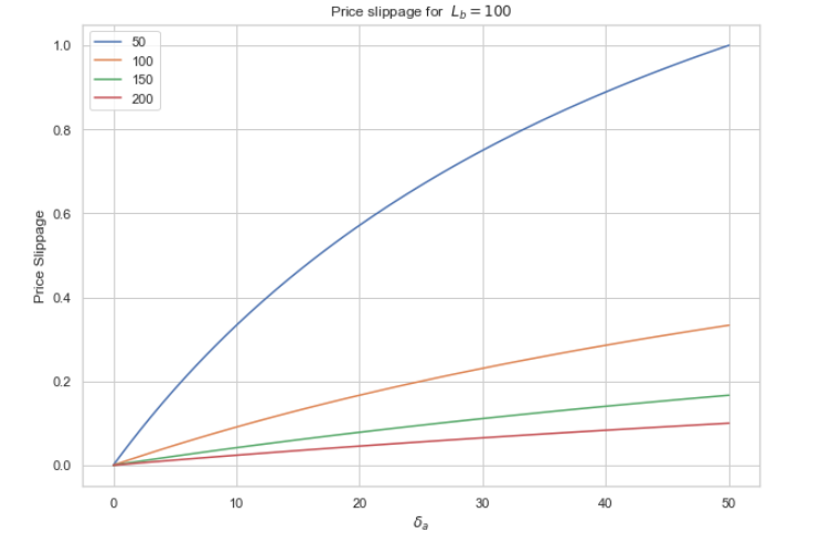
Now, if the size of the sell trade was large, this would mean that the denominator on the right hand side is large, and so the number of tokens in exchange would be less. The difference between this and the market price is called trade slippage.

The graph below shows the trade slippage for different liquidity values of L_a. Of course, if there are more significant amounts of token A in our liquidity pool, the gradient for trade slippage is less.
Uniswap
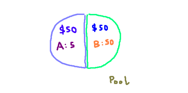
Uniswap is an example of a constant product market maker and was one of the first constant product market makers out there. In the case of Uniswap, liquidity providers need to initially provide equal dollar amounts of the two tokens (although this need not necessarily be the case for other AMMs). For example, suppose token A was worth $10, and token B was worth $1. If the liquidity provider wanted to provide $100 worth of liquidity to the pool, it would mean $50 of liquidity in the form of each token. This means that they would have to commit 5 tokens of token A, and 50 tokens of token B. The diagram below shows this relationship initially.